KOLC+ puts Gaussian splats inside BIM/CIM: how each feature has to work, and how I would build one
mdjsonmcp2026-10-06 · 38 min · 3d · gaussian-splatting · point-cloud · lidar · slam
Why read this
Notabletop 60%Works out what splat volumes, sections and alignment must compute inside a closed BIM tool, then lays out an open, licence-checked pipeline to build one.
- A guide you can follow today
- Original analysis
- A lasting reference
3D & spatialAPI onlyProprietaryPractitioner guide
How this was scored
- Is it new?
- 1 of 3: An incremental tweak
- Can I trust it?
- 2 of 3: Measures key facts from files, code or configs
- Can I run it?
- 1 of 3: API-only, gated or restrictive licence
- Will I understand it?
- 2 of 3: Mechanism from first principles with figures
- Can I act on it?
- 3 of 3: A decision guide a practitioner can follow today
- Will it last?
- 2 of 3: A reference for a year or more
- Does it affect many?
- 1 of 3: A specialist community
- Only here?
- 2 of 3: A teardown or measurement few others did
Score 63 of 100, ranked 183 of 445 rated articles. Each question is answered 0–3 by hand, and a 3 is rare. How articles are scored
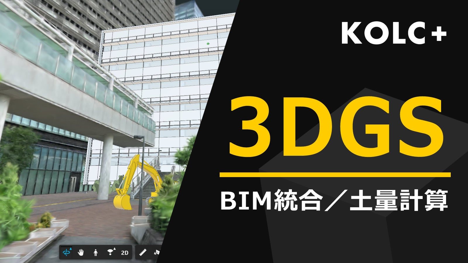
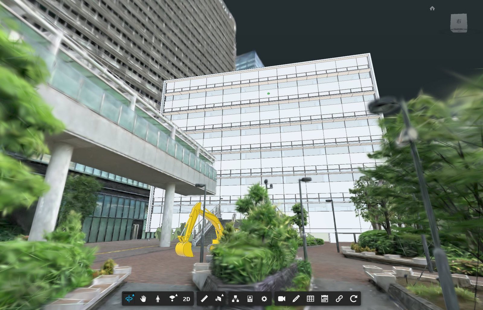
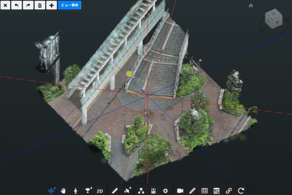
On 6 October 2026 KOLG Inc. (株式会社コルク, Tokyo) announced that the "integrated app" of its BIM/CIM cloud, KOLC+, now takes 3D Gaussian Splatting scenes into the same space as BIM/CIM models, point clouds, terrain and 2D drawings, and that its earthwork, section, placement, annotation and 4D tools work on them (press release, in Japanese). The motivation it gives is concrete: sites have been buying XGRIDS scanners, and someone has to do something with the .lcc files they produce.
A splat next to a Revit model is a nice picture. A splat that a quantity surveyor signs an earthwork volume off is a different object, and the release does not say which one KOLC+ is. It is closed, and no accuracy figure is published anywhere I could find. So this piece reads what KOLG shows (the release, its screenshots, three product pages), works out what each feature has to compute when the input is anisotropic Gaussians rather than a surface, and then builds the same thing from open parts on the stack I would use: a 360 camera, Spirula Studio, gsplat, Revit.
Labels, as everywhere on this site: reported is KOLG's or a project's own claim; measured is something I read off a file, a screenshot or a spec; reasoned is my arithmetic on the other two.
What was announced
The feature list in the release, translated, with what each item has to compute once the input is a splat. Everything in the first two columns is reported.
| KOLC+ feature (release) | What it shows | What it has to compute on splats |
|---|---|---|
| Integration with BIM/CIM, point clouds, terrain, 2D drawings, measurement data, GNSS | Revit model over an XGRIDS splat | a common coordinate frame and a shared depth buffer |
| Alignment, 3-point matching | move/rotate gizmo; public-coordinate data placed automatically | a similarity transform from three correspondences |
| Earthwork volume (BIM vs splat, or two epochs of splats) | "surface determination from 3DGS alone" | a height field from something that is not a surface |
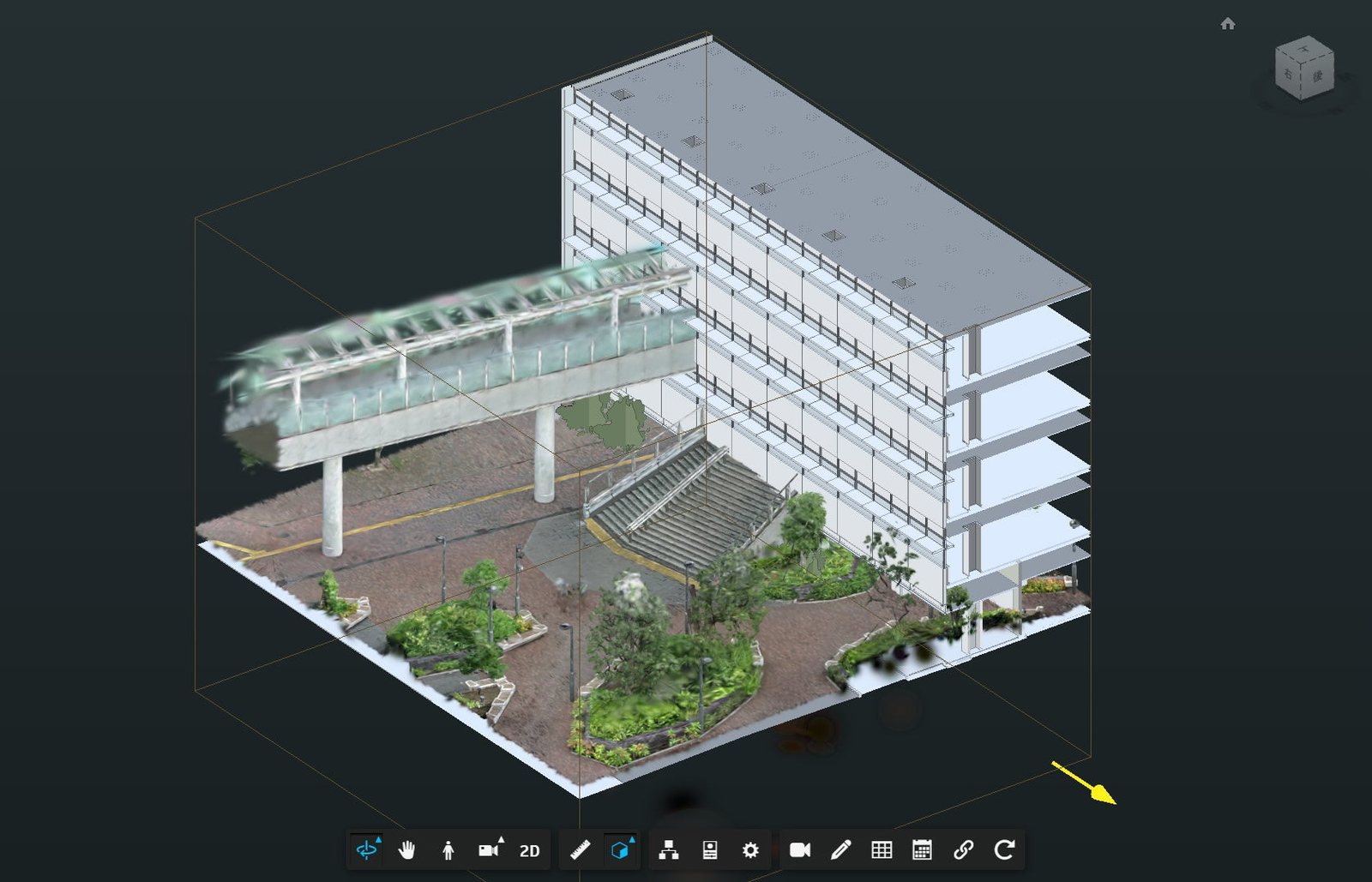
| Sections: auto-trace, manual trace, DXF out | stair profile traced as a polyline | the intersection of a plane with millions of Gaussians |
| Section box (6 faces), slices | BIM-vs-splat clash check | clipping splats by planes in the renderer |
| Measurement: coordinates, distance, angle, area | coordinates in metres to three decimals | a 3D point under the cursor |
| Spatial notes, markup | labels pinned in the scene | the same picking |
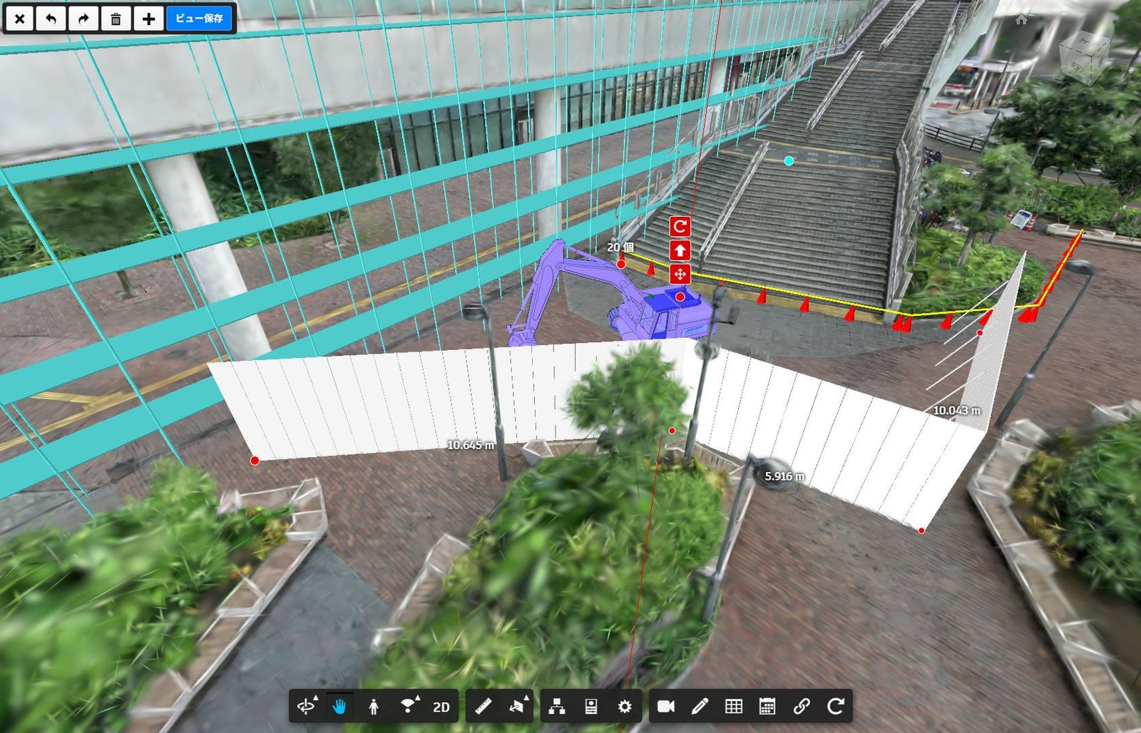
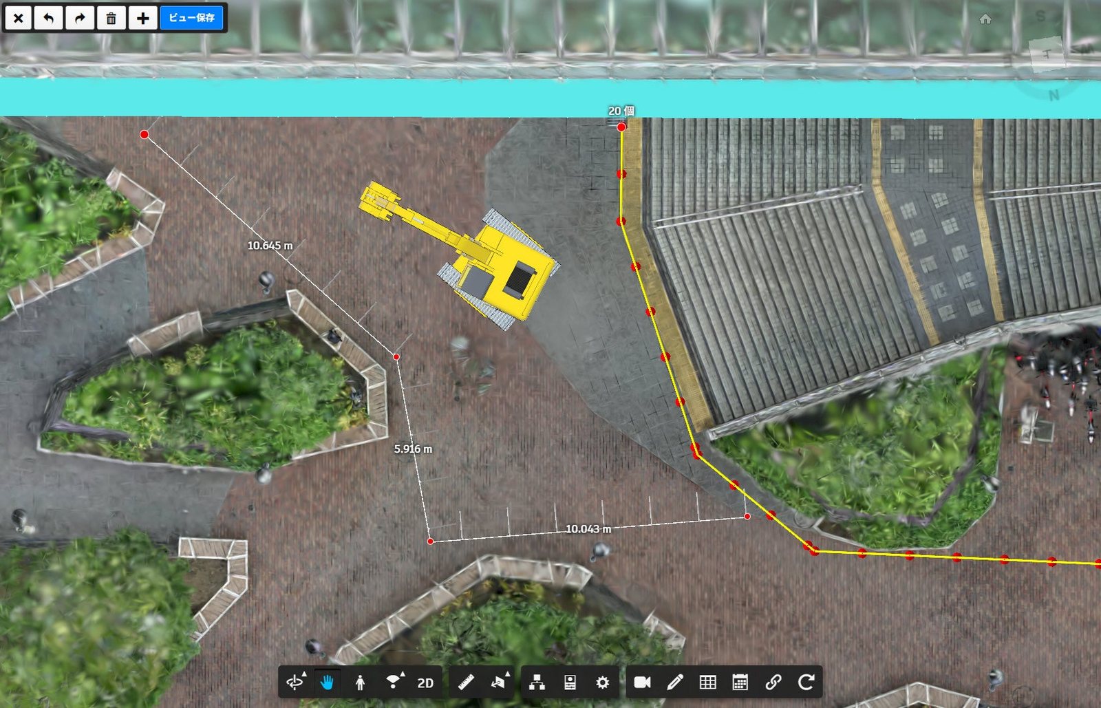
| Placement planning: scaffolding, hoarding, sandbags, cones | excavator and fence placed on the plaza | ground height under a dragged object |
| 4D timeline, walkthrough, saved views | none shown | time-indexed visibility; camera paths |
| "Point-cloud mode" toggle for 3DGS | splat centres as coloured points | the Gaussians' means, drawn as points |
Formats and money, also reported: the integrated app reads LCC (.lcc) only, exported by XGRIDS' free LCC Studio; "LCC2, PLY, SPZ and others" are "under consideration". That is narrower than KOLC+'s separate 3DGS viewer, whose product page lists PLY (compressed and uncompressed), SPZ, SPLAT, KSPLAT and SOG with LoD streaming, says PLY is converted to "1/8" of its size for delivery, and until this release said the integrated app could only show a splat in a split screen beside the model (3DGS viewer page). The price is ¥50,000 a month before tax for 100 GB, 100 users and the integrated app on two sites, with no setup fee. The pricing page shows where that comes from: the ¥30,000 3D plan plus the integrated-app add-on at ¥10,000 per site, minimum two (reasoned: 30,000 + 2 x 10,000 = 50,000). KOLC+ is also registered as an information-sharing system (ASP) for MLIT work and reports 500+ companies using it. KOLG shows it at Construction Technology Expo 2026 Kanto, 20-21 October, Sunshine City in Ikebukuro, booth B-61.
A splat is not a surface
Everything hard in that table comes from one fact. Each Gaussian is a mean , a covariance , an opacity and a colour, and the optimiser was paid to make images match, not to put mass on surfaces. Most mass ends up near surfaces anyway. Some does not: floaters in front of glass, haze in the sky, flat Gaussians painting a road's texture a few centimetres off the asphalt, a shell around foliage. So every geometric query must answer "where is the surface along this ray?", three ways:
- The first Gaussian the ray enters, at some -sigma ellipsoid, with an opacity floor. Cheap, and wrong whenever a floater sits in front.
- The expected depth, with the usual compositing weights . Smooth, and biased toward the background at edges, where it averages a foreground and a background into a depth that is neither.
- The median depth, the at which accumulated opacity crosses 0.5. It does not average across a silhouette. The 2DGS paper uses median depth for its meshes and reports that expected depth reconstructs worse; Gaussian Opacity Fields goes further and extracts the level set of an opacity field directly.
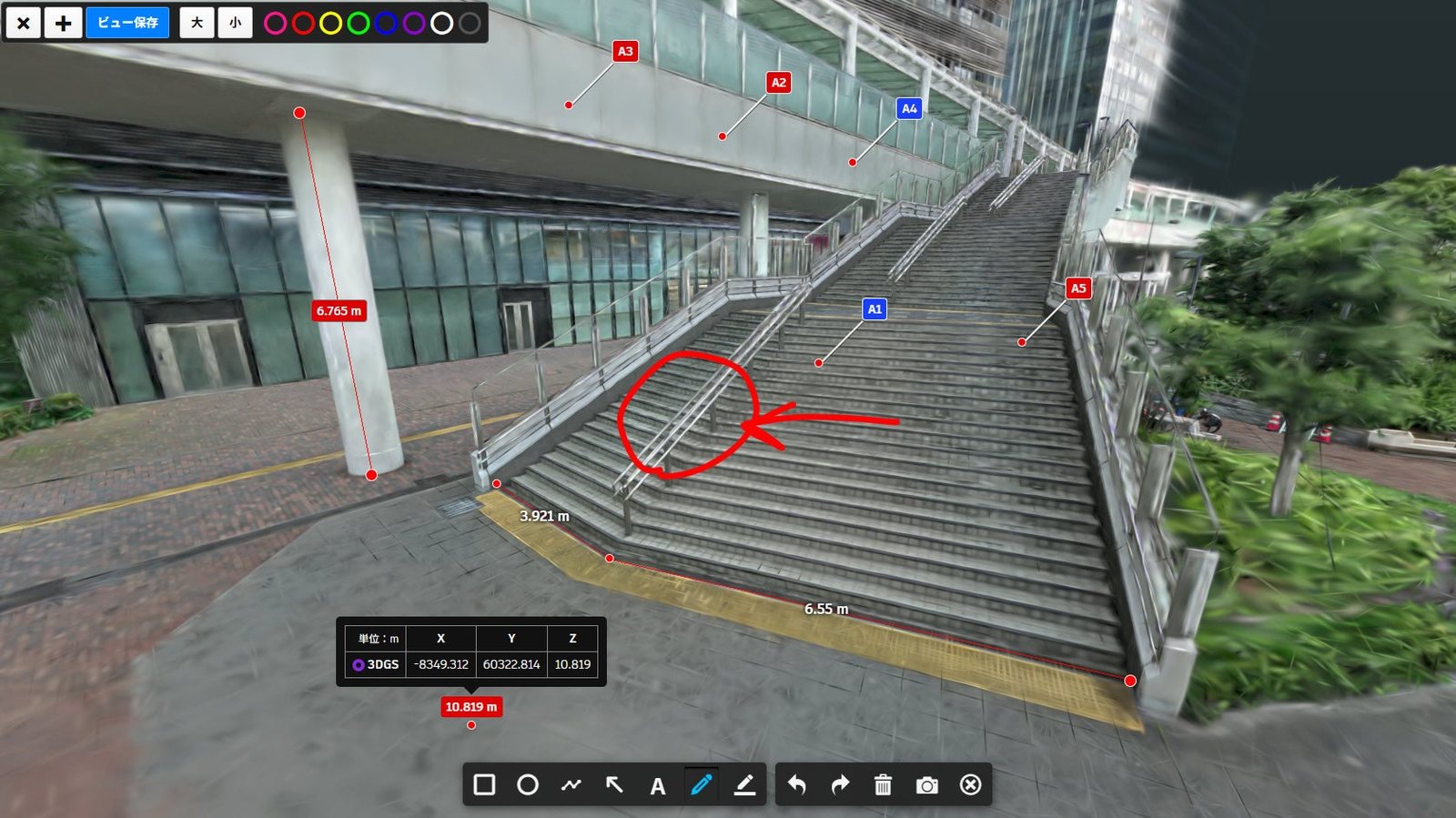
KOLG's release says its measurement and annotation tools use "an in-house hit-detection logic" that makes raycasting fast and coordinate detection precise, and that the point-cloud mode lets you "check the state of the hit detection". The viewer page adds that its distance tool judges "the contact point between the Gaussian-distribution mesh and the mouse cursor" (reported, my translation). That reads like the first option: a proxy mesh of ellipsoids at a fixed sigma, ray-cast on the CPU or with a BVH. It is the fast answer. I cannot see the opacity floor or the sigma, so I cannot say how it treats floaters.
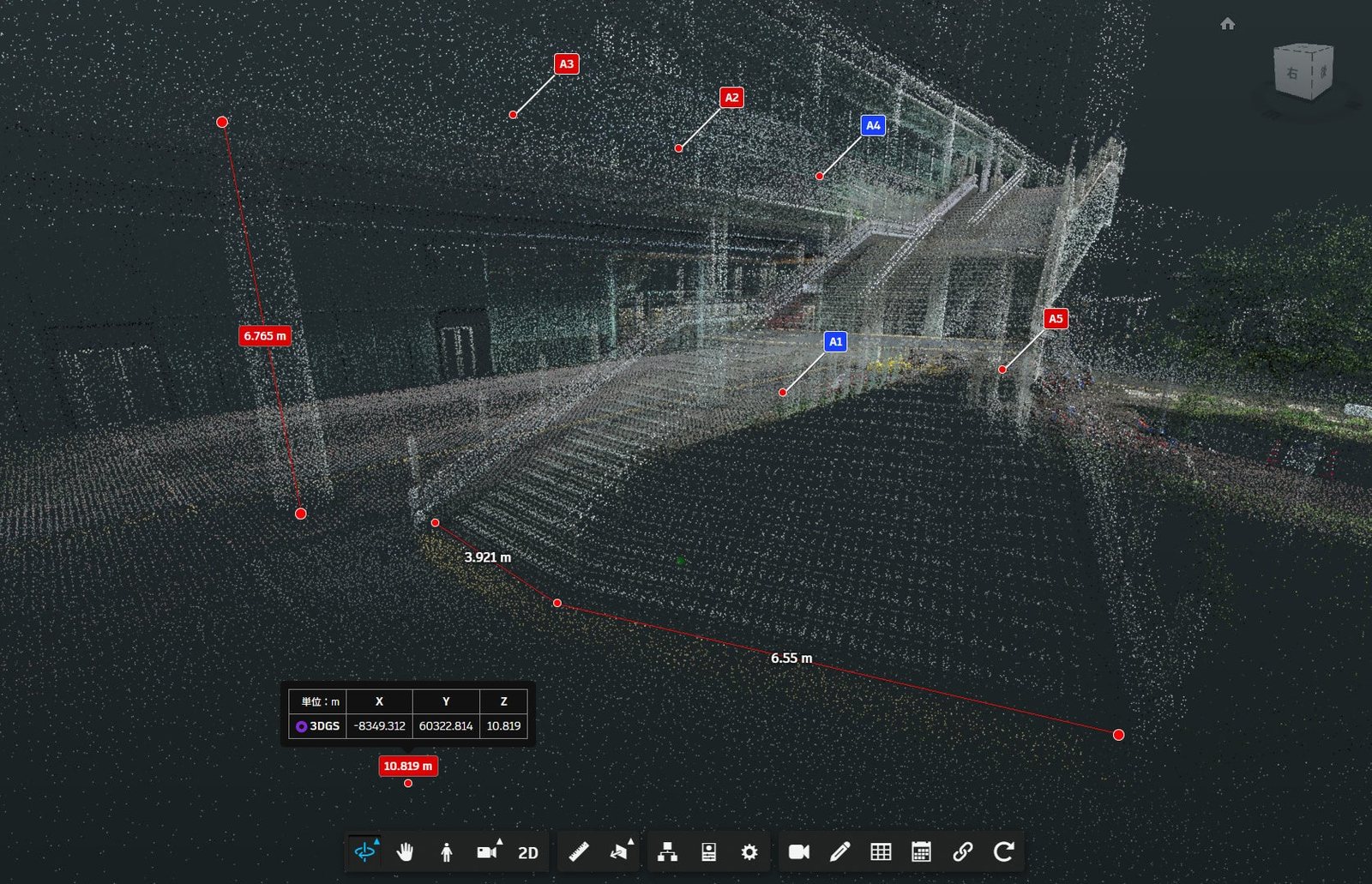
The point-cloud mode is honest about the representation: sparse on flat ground, dense on edges and texture, because a splat's centre density follows image gradients where LiDAR's follows range and incidence. The centres are not samples of the surface; they are the centres of blobs whose extent you are throwing away.
What splat geometry is worth, measured by other people
No one has published accuracy for KOLC+. Several groups have published it for splats against survey references, and the pattern is consistent (all reported, each paper's own tables):
| Study | Capture | Reference | Result |
|---|---|---|---|
| McNally et al., ISPRS Annals 2026 | phone on a gimbal, two building exteriors | total station + TLS | targets picked in the splat: 0.8-1.9 cm RMSE; Gaussian centres as a cloud: 3.6-13.6 cm mean distance, decimetres RMS from floaters |
| Clini et al., ISPRS Archives 2024 | Insta360 X4, church interior | Leica RTC360 | splat mean error 6 mm, but standard deviation 25.8 cm |
| Suwardhi et al., ISPRS Archives 2026 | GoPro MAX 360 video, heritage building | Leica BLK360 | control residual 12.5 cm RMS; cloud-to-cloud mean 15.2 cm |
| Haitz et al., ISPRS Annals 2024 | nadir aerial, about 2 cm pixels | airborne LiDAR | splat centres 0.28-0.40 m RMSE; COLMAP MVS 0.07-0.09 m |
| LI-GS | two Hesai XT32 + an Insta360 | the rig's own LiDAR | LiDAR-constrained surfels 4.51 cm; image-only 2DGS, GOF, PGSR 14.8-16.6 cm |
Read it as three statements. A splat built on a well-controlled SfM solve keeps the solve's geometry: McNally's targets moved less than 8 mm between the SfM input and the splat. Reading the Gaussians as a point cloud is several times worse than that, mostly because of floaters. And a 360 camera alone sits at decimetres, while LiDAR constraints bring a splat to about 5 cm, measured against the same LiDAR. I found no peer-reviewed study that validates an earthwork or stockpile volume computed from splats.
Earthwork volumes from two epochs
What KOLC+ computes
KOLC+'s earthwork page is specific (reported, translated): volumes are computed by the point-height method (one-point method) in MLIT's civil-works quantity rules (土木工事数量算出要領), which "computes the elevation difference at the mesh intersections"; the rules call for a mesh of "50 cm or less", KOLC+ lets you set any size; and a "median" mode reduces point-cloud noise. The reference and comparison surfaces can be a TIN drawn in the viewer, BIM/CIM, LandXML, FBX/OBJ, point clouds, GSI terrain, or all models together. The release adds two epochs of 3DGS to that list, and says the surface determination runs "on 3DGS alone".
The one-point method is the simplest volume integral there is. On a grid of cell area :
where and are the reference and comparison heights sampled at grid node . All the difficulty is in and .
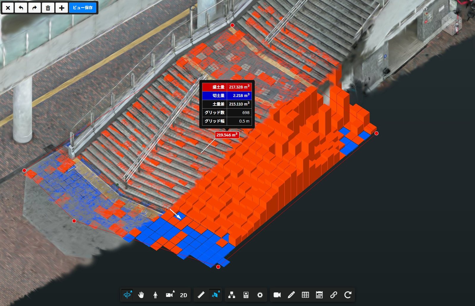
Read off the screenshot (measured): fill 217.328 m³, cut 2.218 m³, difference 215.110 m³, 698 cells of 0.5 m, and a label of 219.546 m³, which is fill plus cut. So the area is 174.5 m² and the net averages 1.23 m (reasoned). The fill columns rise over a staircase: this measures the stairs above some reference surface the release does not name. It demonstrates the tool; it is not a validated quantity.
Turning a splat into a height field
There are four ways to get from a splat, in increasing order of effort.
- Centres as points, filtered. Drop Gaussians below an opacity floor and above a size limit, then take the lowest, median or highest centre per cell. Fast, and what a "point-cloud mode" plus the median option would naturally do. It is also biased: at object scale, Petrovska and Jutzi found every radiance-field method's points sat inside a statue's surface on average, by 1.6 to 3.5 mm in the clear scene, while MVS sat 0.16 mm outside (reported). Scaled up to a stockpile, a surface that sits inside reads as missing volume.
- Depth renders from above. An orthographic median-depth map straight down, per epoch, is a DEM directly. Overhangs and canopy go into it.
- A surface-trained model. Train with a method that puts Gaussians on surfaces: 2DGS flattens each Gaussian into a disc with a normal; Gaussian Opacity Fields (GOF) and PGSR add depth-normal consistency and extract a mesh. Then rasterise the mesh. More training work, much better geometry. The 2DGS paper's own ablation on DTU shows the order: 3DGS centres meshed with Poisson 1.65 mm Chamfer, 2DGS expected-depth fusion 0.88, median-depth fusion 0.80 (reported). Fused depth beats centres; median beats mean.
- Do not use the splat for geometry. An XGRIDS export ships a LAS beside the splat. Boring, and for a payment quantity, right.
Whichever route, the errors are the same:
- Floaters add spikes, almost always as fill. A median per cell removes isolated ones; a sheet of haze is not isolated.
- Vegetation: the splat models the canopy, and has no second return to see under it. It needs ground classification as LiDAR does.
- Scale: a scale error scales every length by , so volumes by , about . Spirula's notes report about 0.2% scale from GPS over a 100 m walk; that is about 0.6% of volume (reasoned).
- Registration between epochs, the big one.
How registration error becomes volume error
Let epoch 2 be registered to epoch 1 with a small vertical offset and a small tilt about a horizontal axis through the point . To first order the height error at horizontal position is , where is the horizontal direction perpendicular to the tilt axis. Integrate over a region of area with centroid :
Two consequences (reasoned):
- The offset is linear in area and does not average out. On the screenshot's 174.5 m², every centimetre of is 1.745 m³, 0.8% of its 215.110 m³. On a 1 ha cut, a centimetre is 100 m³.
- Tilt nets to zero only over a region centred on the pivot. Over any region off to one side, it is a bias. And even when it nets to zero, it moves volume between cut and fill: the gross numbers both grow, which matters when cut and fill are paid separately.
A tilt comes from the targets you aligned on. One target 2 cm off vertically on a 30 m baseline tilts the fit by about 0.67 mrad (0.038°), which is 1.3 cm of height 20 m from the pivot (reasoned). Two centimetres is an ordinary RTK fix; a thin lift is not much more.
The widget runs the one-point method on a synthetic 40 m x 30 m site, where epoch 2 adds a pit (cut) and a stockpile (fill).
| m³ | truth | measured |
|---|---|---|
| cut | 198.5 | 198.5 |
| fill | 112.9 | 112.9 |
| net | -85.6 | -85.6 |
| net error | 0.0 |
A dz of 0 cm over 1200 m² is 0.0 m³ of net error by itself. Tilt about the centre nets to zero but still inflates cut and fill separately.
On the 0.5 m grid (reasoned, synthetic): the truth is 198.5 m³ cut and 112.9 m³ fill. A 5 cm offset over 1,200 m² moves the net from -85.6 to -25.6 m³, exactly 60 m³. A 0.10° tilt about the centre leaves the net at -85.6 but raises cut to 208.8 and fill to 123.2. Floaters add fill; the 3x3 median takes almost all of it back.
Would it count?
In Japan the question has a precise answer, because MLIT writes the test down. The March 2026 edition of its as-built control rules for 3D measurement (「3次元計測技術を用いた出来形管理要領(案)」, PDF) sets the same accuracy classes for earthwork surfaces whether the instrument is a UAV camera, a terrestrial scanner, a mobile scanner or ground photogrammetry (measured, read in the text):
| Purpose | Accuracy, vertical and horizontal | Point density | Ground pixel size (photo methods) |
|---|---|---|---|
| Pre-construction survey, rock line | ±100 mm | 1 per 0.25 m² (0.5 m mesh) | 20 mm/px or finer |
| Interim payment quantities | ±200 mm | 1 per 0.25 m² | 30 mm/px or finer |
| As-built | ±50 mm | 1 per 0.01 m² to measure, 1 per m² to evaluate | 10 mm/px or finer |
Accuracy is proven per site on check points against known coordinates, and the record is submitted; the pixel rule can be relaxed if that check passes. Deliverables are the point cloud (CSV, LandXML or LAS) and TIN surfaces as LandXML. A .lcc or .ply is not on the list, though methods the rules do not describe may be agreed with the client site by site.
So, on my reading, a splat volume counts only if the geometry under it passes the ±50 mm or ±200 mm check-point test and is delivered as points and a TIN, or the client agrees for that site. KOLG claims neither. For a 360 camera, the pixel rule is arithmetic (reasoned): an 8K ERP spreads 7,680 px over 2π, so a pixel covers , reaching 10 mm at about 12.2 m. Against the published numbers above (12.5-25.8 cm for 360-only captures), ±50 mm needs LiDAR or very good control.
Sections and DXF from Gaussians
Slicing a Gaussian with a plane
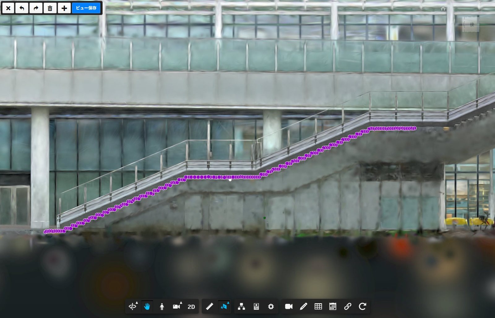
KOLC+'s section tool traces a profile automatically between two picked points, lets you edit the traced vertices, and exports DXF as 3D lines in public coordinates or flattened to the XY plane, with one layer per model (reported, section tool page). On a point cloud you take the points within a slab around the plane and trace them. On splats there is a closed form.
Take the plane through with unit normal , and an orthonormal basis () for it, so a point on the plane is with . Write and , the signed distance from the Gaussian's mean to the plane. The Gaussian's density along the plane is
The exponent is a quadratic in , so the slice is a 2D Gaussian. Completing the square:
The last term is the minimum of the Mahalanobis distance over the plane, a standard result for conditioning a Gaussian on a linear constraint. Three things fall out:
- The cut of the -sigma ellipsoid is an ellipse with centre and shape matrix : . It exists only when , so a cull is one dot product per Gaussian: is the Gaussian's standard deviation along the plane's normal.
- The slice's density is a 2D Gaussian with covariance and peak weight . A Gaussian lying flat in the plane contributes fully; one whose mean is two normal-sigmas away contributes of its opacity.
- is the Schur complement , so you never need to invert the 3x3 covariance at all.
A section is then an image: splat every surviving Gaussian's 2D slice onto a raster in plane coordinates, each with its weight, and you have an opacity field on the section plane. The profile is the 0.5 contour of accumulated opacity (marching squares), or the ridge of the density. That polyline goes out through ezdxf as an LWPOLYLINE in the plane's 2D frame or a 3D POLYLINE mapped back through into site coordinates. For the "public coordinates" option, keep the coordinates in float64 all the way to the file; the next section shows why float32 is not enough.
The section box is the same test, , against six faces, plus a per-fragment test so a straddling Gaussian is cut along the plane rather than popping in and out whole.
Registration: three points, and why that is a minimum
KOLC+ offers a manual move-and-rotate tool, "3-point matching" to a BIM model, and automatic placement for data already in public coordinates (reported).
Three-point matching is a similarity transform : rotation (3 parameters), translation (3) and scale (1). Seven unknowns. Each correspondence gives three equations. Two points give six, and leave the rotation about the line through them free. Three non-collinear points give nine, two more than needed. The least-squares solution is Umeyama's (1991): with centroids , variance of the source points and cross-covariance ,
guards against a reflection; fix for a rigid fit. COLMAP's model_aligner does the same from camera centres and needs "at least 3 images".
Three points is the minimum to solve, not to check. With exactly three, every point is fitted and the residuals tell you nothing; with five, two of them are independent check points, and their residual is the honest number. Geometry matters as much as count. Points that are nearly collinear leave the rotation about their line weakly determined, and Spirula Studio's LiDAR notes measured exactly that: a centres-only Umeyama fit was 1.9° off the anchors' own rotations "on the FJD walk, which is nearly a line -- the rotation about it is free"; fitting rotations first, from the anchors' poses, gave 0.16° (reported, docs/notes/lidar-alignment.md). Points on one plane, say all on the ground, leave tilt determined by their vertical errors over their spread, which is the 0.038° from the previous section.
Layout matters more than count. I simulated it (measured, 4,000 Monte Carlo trials of an Umeyama fit, 2 cm noise per axis on both the picked and the surveyed coordinates, a 100 m square site). The vertical error at the centre and at the far corner: three corners, 2.0 and 5.0 cm; four corners, 1.4 and 2.4 cm; four targets clustered in one 20 m corner, 7.9 and 17.6 cm. Targets have to surround what you measure. Better still, put them into the bundle adjustment as control, so the poses themselves are in the survey frame and the solve's own bending is corrected, which no seven-parameter fit afterwards can do.
Then refine. Point-to-plane ICP against a LiDAR scan, or against the BIM model's own floor and wall faces where the as-built is expected to match, takes out the residual tilt and scale that the targets leave. It needs a starting point inside its basin: Spirula measured convergence from about 5° and 10% scale, failure at about 10° (reported). Three points get you there; ICP finishes it.
The LCC container
KOLC+'s integrated app reads only .lcc (Lixel CyberColor). XGRIDS publishes the layout in an LCC white paper (read at b38c2eb). A scene is a folder: meta.lcc (JSON), Index.bin, Data.bin, and optionally Shcoef.bin (higher-order SH), Environment.bin (far background) and Collision.lci (a mesh with a serialised BVH).
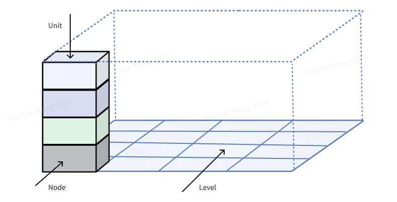
It is a 2D tiling with a LOD pyramid per tile: a Unit is a grid cell (x and y packed into a uint32), a Node is that cell at one level, and Index.bin gives each node's splat count, offset and size in Data.bin, so a viewer streams the right level per tile. The base record is 32 bytes (measured, white paper table):
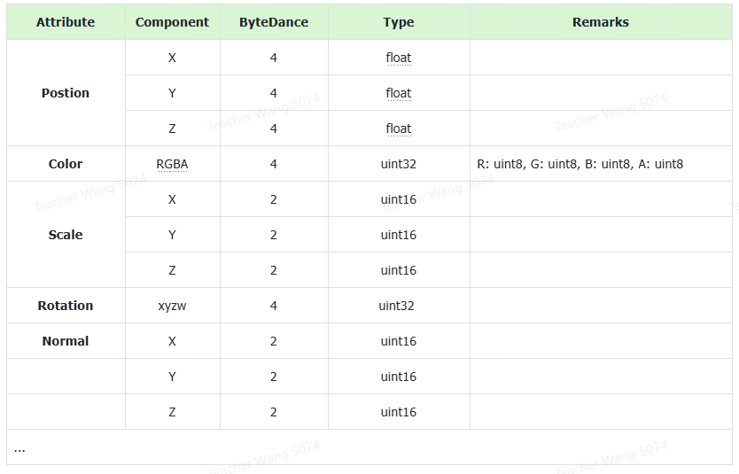
Position is three unquantised float32 (12 bytes), colour RGBA8 with opacity in alpha (4), scale three uint16 dequantised between per-scene bounds (6), rotation one uint32 in smallest-three 10-10-10-2 packing, the trick SOG and SPZ also use (4), and a normal as three uint16 (6). The Portable profile stops there. Quality adds 64 bytes in Shcoef.bin, the degree-1 to 3 coefficients as fifteen RGB triples packed 11-10-11. So 96 bytes a splat against 248 for a float32 PLY at SH3, 2.6x smaller before any LOD (reasoned).
The LOD is not free. The white paper's example meta.lcc lists nine levels with 2,890,271 splats at LOD0 and roughly 0.47x fewer at each level down; summed, all levels hold 5,440,665 splats, 1.88x the finest level (measured from the example). If every level is stored, a Quality LCC is about 96 x 1.88, roughly 181 bytes per finest-level splat, only 1.4x smaller than the PLY (reasoned). The example does not add up, either: its totalSplats says 3,678,719 "include all lods", and its indexDataSize of 86 bytes does not match the 4 + 9 x 16 = 148 the index table implies for nine levels (measured). Do not use it as a test vector.
Two details matter for construction. First, float32 positions in public coordinates lose millimetres. A float32 has a 24-bit significand; at the Y = 60,322.814 m in the KOLC+ screenshot, adjacent representable values are 2^-8 m, about 3.9 mm, apart (reasoned). That is why the metadata carries a global offset, shift, scale and epsg: store local coordinates, keep the georeference in float64 beside them. A pipeline that writes public coordinates straight into a float32 file quantises its own survey. Second, the licence is conditional: a visible "Data Organization Format originated from XGRIDS" attribution in your product, derivatives under terms "no less open", no use of the format to train AI models that compete with XGRIDS, and arbitration in Shenzhen under PRC law (reported, white paper sections 4-5). Reading .lcc is easy; building a product on it is a contract.
The open formats, and the one I would pick
You do not need LCC to leave XGRIDS' world. PlayCanvas's MIT-licensed splat-transform reads .lcc and .lcc2 and writes PLY, SPZ, SOG, streamed SOG and glTF (reported, README). Spirula Studio v2026.10.6 opens an LCC Studio developer_data/ export directly: its raw/ and perspective/ folders are COLMAP datasets in the frame of the scanner's LAS (reported, docs/notes/lidar-alignment.md).
| Format | Owner, licence | Positions | Compression | LOD / tiling | Read by |
|---|---|---|---|---|---|
| PLY (3DGS layout) | Inria reference layout, de facto open | float32 | none; 248 B a splat at SH3 | none | everything |
| SPZ | Niantic, MIT | 24-bit fixed point, 12 fractional bits by default | quantised + zstd (v4) | none | Spark, PlayCanvas (via splat-transform), Niantic tools, KOLC+ viewer |
| SOG / streamed SOG | PlayCanvas, MIT | 16-bit, log domain per axis | WebP images, codebooks; 18x on the bicycle scene | streamed SOG: chunked LOD (lod-meta.json) | PlayCanvas engine, SuperSplat, Spark, KOLC+ viewer |
glTF + KHR_gaussian_splatting | Khronos, ratified | float or normalised ints on a point primitive | none in the base extension | via 3D Tiles (glTF content) | CesiumJS and the Khronos ecosystem |
| LCC | XGRIDS, white-paper licence with conditions | float32 + global offset/EPSG | 32 B (Portable) or 96 B (Quality) | 2D grid of units, LOD pyramid per unit | XGRIDS tools, KOLC+ integrated app, splat-transform (read) |
Two reasoned consequences. SPZ's 12 fractional bits on a 24-bit integer give a 0.24 mm step over plus or minus 2,048 m, so a public coordinate like 60,322 m needs a local origin. SOG's log-domain 16 bits spend precision near the origin, so put the origin mid-site, not at a monument a kilometre away.
KHR_gaussian_splatting is now "Complete, Ratified by the Khronos Group" (measured, its README; the status changed on 3 September 2026). Splats are attributes on a glTF point primitive, which degrades to a point cloud in a viewer that does not know them, and since 3D Tiles content is glTF, it is the path to splats in a geospatial tileset. Compression is left to follow-on extensions, the SPZ one still an open proposal.
My pick for a web viewer that overlays IFC: streamed SOG on the PlayCanvas engine. MIT end to end, LOD streaming already there, a converter that reads everything above including .lcc, and files small enough to ship an epoch a week. The IFC goes through That Open's web-ifc (MPL-2.0), or is converted to glTF into the same scene; one renderer and one depth buffer is the requirement, not the library. If the deliverable is a georeferenced tileset over terrain, glTF splats in 3D Tiles on CesiumJS is the standards answer, with bigger files for now.
Building a KOLC+-like pipeline from open parts
KOLC+ starts after capture and SfM: the splat arrives from XGRIDS trained and posed. A pipeline you own has to do those too. Here is the one I would build around a 360 camera. Licences are as I read them in each repository's LICENSE, COPYING or README this week; an engineer's reading, not legal advice.
- pick
- DJI Osmo 360 or Insta360 X5, 8K equirectangular video; printed AprilTags plus surveyed targets
- or
- a LiDAR + camera rig (XGRIDS-style) where the earthwork tolerance demands it
- in → out
- .OSV / .insv → ERP .mp4, GCP list in the site CRS
- licence
- hardware; GCPs shot with RTK GNSS or a total station
- KOLC+
- KOLC+ does not capture. The press release says customers scan with XGRIDS and export .lcc from LCC Studio.
Put at least five targets around the perimeter and at two heights. Three is the minimum for a similarity; the extra ones are your check points.
1. Capture
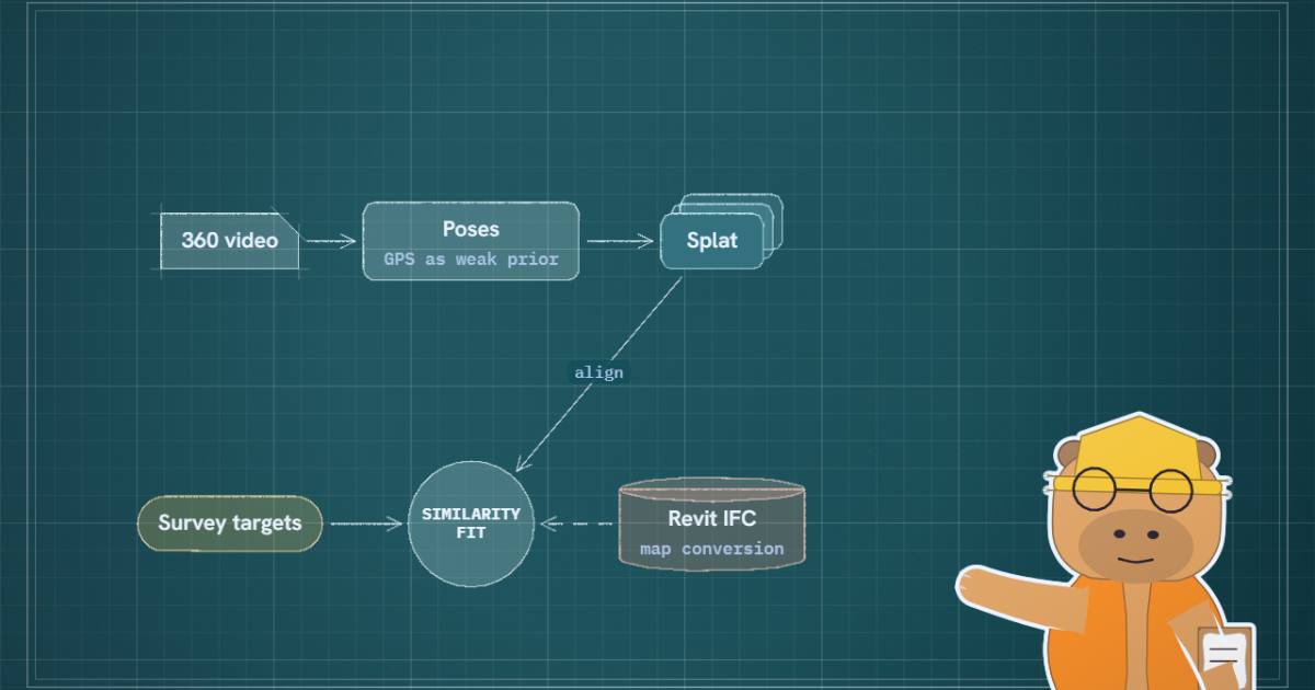
A DJI Osmo 360 or Insta360 X5, walked or flown, recorded at 8K. Stitch to equirectangular (ERP) in DJI Studio or Insta360 Studio before SfM, for the reason the capture-pipeline piece established: a dual-fisheye file makes the solver discover the rig, and on long captures it fails to. Turn in-camera horizon levelling off if you mask the stitch seam.
The camera's GPS is a phone's, pushed over Bluetooth, good to metres. Put out five or more targets around the perimeter and at two heights and shoot their centres with RTK GNSS or a total station: three for the fit, the rest as check points. Where the tolerance is tight, add a LiDAR scan.
2. Poses: Spirula Studio, or COLMAP
Spirula Studio solves the ERP as one spherical camera, takes GPS as a weak per-frame prior with a Huber loss, and since v2026.10.6 takes a laser scan as an input next to photos and videos: E57, LAS 1.0-1.4 (uncompressed; LAZ is refused) or PLY (reported, docs/notes/lidar-alignment.md). SfM still runs; then a similarity fit (rotation from anchor images, RANSAC scale and translation, point-to-plane ICP) moves the model into the scan's metric frame, the scan thinned to 500k points seeds the Gaussians, and depth and normal maps rendered from it replace the monocular ones. It is marked experimental. As the update to the Spirula piece found in the code, the depth loss is off by default and is a scale-blind Pearson correlation when on, so the metric accuracy comes from the alignment and the seeds, not from a depth loss.
Its own measurements are the best public evidence I have seen for 360 video plus LiDAR (reported, the project's note, 4 October 2026):
| Capture | Anchor fit | After ICP |
|---|---|---|
| FJD Trion P2 E57 (51 panoramas) + Insta360 X5 video (224 frames) | 0.16° / 3.5 cm | 1.3 cm to the surface |
| Same LAS without photos + the same X5 video | 0.16° / 1.1 cm | 0.8 cm |
| ETH3D courtyard, DSLR + FARO scan | 0.14° / 2.0 cm | 3.0 cm / 0.11° vs ground truth |
| Oxford Spires, 525 handheld images + 19 RTC360 scans | 0.59° / 36 cm | 12.8 cm |
The last row is the useful one: when photographs and scan barely overlap, it says so with a big number. Spirula is GPLv3: fine as a separate process, a conversation with a lawyer if you link it into a product.
The permissive alternative is COLMAP (BSD-3-Clause): EXIF GPS becomes pose priors for its pose_prior_mapper, GLOMAP is now its "global" mapper, panorama_sfm.py turns 360° images into a virtual pinhole rig, and model_aligner fits the similarity to GCPs (reported, COLMAP docs). Feed-forward pose models are improving fast (the first and second roundups), but read the weights' licences: MASt3R is CC BY-NC-SA 4.0, and of VGGT's checkpoints only the gated VGGT-1B-Commercial allows commercial use.
3. Training: gsplat for licence, 2DGS for geometry
For appearance any trainer works. For a pipeline that measures, two constraints decide it.
Licence. The reference code for 3DGS, 2DGS and Gaussian Opacity Fields carries Inria's licence: "THE USER CANNOT USE, EXPLOIT OR DISTRIBUTE THE SOFTWARE FOR COMMERCIAL PURPOSES" (measured, each LICENSE.md); PGSR's is "educational, research and non-profit purposes only". gsplat is Apache-2.0 and ships its own 2DGS rasteriser, the commercial-safe route to surfel geometry; mesh it with your own median-depth TSDF. LichtFeld Studio and Spirula are GPLv3.
Geometry. Train one appearance model and, if you need measured surfaces, one surface model, or use the LiDAR for geometry outright. The trained splat is for the viewer; the DEM and the sections come from the scan or the 2DGS mesh. Mixing the two roles is how floaters end up in a payment quantity. Spirula's new region-of-interest editor keeps the training budget on the site without cropping the scene: densification outside the region is weighted by 1e-4 (reported, the Spirula update).
4. Georeferencing
Fit the similarity from the GCPs (Umeyama, above), report residuals on the check points, then ICP against the scan. If there is no scan, ICP against the BIM's floor slabs and core walls in areas you expect to be as designed. Choose the target CRS once. In Japan that is a JGD2011 plane rectangular zone; everywhere, keep the coordinates as float64 offsets from a site origin and the origin plus EPSG code as metadata.
5. Revit to the same frame
This is where splat-plus-BIM demos quietly cheat, by dragging the model until it looks right. Revit has three points:
- Internal origin: fixed, the origin of the model's own coordinates. Revit warns when geometry is more than 20 miles (about 32 km) from it, and snapping and graphics degrade well before that (reported, Autodesk help). Japanese plane-rectangular coordinates are routinely tens of kilometres, so never model at public coordinates.
- Project base point: a reference the team chooses, usually a grid intersection.
- Survey point: the link to the world. Through shared coordinates it carries an easting, northing, elevation and the angle to true north.
The georeference that matters is the survey point plus the true-north angle: the site's shared coordinates. Acquire them from a georeferenced site model or specify them at a surveyed point, and check against a monument before exporting anything. In Japan, check the height datum too: the JGD2024 survey results that took effect on 1 April 2025 changed only heights, by up to tens of centimetres on control points, so a design surface and a new scan can disagree vertically before anyone has moved any earth (reported, GSI).
Then export IFC with Autodesk's open-source exporter (revit-ifc, LGPLv2). Its coordinate bases are the SiteTransformBasis enum: Shared, Site, Project, Internal, ProjectInTN, InternalInTN (measured, CommonEnum.cs). Export IFC4 with an EPSG code set and it writes an IfcMapConversion with eastings, northings, height and the true-north rotation, leaving the world coordinate system at zero; IFC2x3, or no EPSG code, bakes the offsets into the placement instead (measured, Exporter.cs: "In IFC4 onward and EPSG has value (IfcMapConversion will be created), the wcs will be (0,0,0)"). The first is what you want: the geometry stays local and the reader applies the conversion in float64.
One more trap, reasoned: a projected CRS has a scale factor. In a JGD2011 plane rectangular zone the grid scale is 0.9999 at the origin meridian, so grid distances and ground distances differ by about 1 cm per 100 m there, and differently elsewhere in the zone. A splat georeferenced from GNSS sits in grid coordinates; a Revit model built at true size sits at ground scale. IfcMapConversion has a Scale attribute for exactly this. On a 200 m building it is a 2 cm misfit at the far end, invisible in a demo and very visible in a deviation map.
For the element link, the IFC already has what you need. The exporter fills each element's Tag with its Revit ElementId by default, and its GlobalId from the element's IfcGUID parameter when present, with an option to store the generated one back into Revit so it stays stable between exports (measured, NamingUtil.cs and GUIDUtil.cs). IfcOpenShell (LGPL-3.0) iterates the geometry into per-element meshes keyed by GlobalId, with the category (IfcWall, IfcSlab, …) and property sets alongside. Autodesk Platform Services' Model Derivative API is the paid cloud alternative, and can itself produce IFC from an RVT.
With elements in the splat's frame, the useful construction queries are per element:
- As-built deviation: sample the surface you trust (LiDAR points, or the 2DGS mesh) inside each element's bounding box, compute the signed distance to the element's faces, and report a histogram per
GlobalId. A wall 3 cm out of plumb is a property ofIfcWall#1234, not a red blob. - Progress on a timeline: for each element, the fraction of its visible faces that have observed surface within tolerance at epoch . Plot that against the 4D schedule's planned date.
6. Earthwork
Per epoch: classify ground in PDAL (filters.smrf or filters.csf) on the LiDAR or the fused splat surface, rasterise with writers.gdal at 0.5 m, difference with rasterio and numpy, and sum with the one-point formula. The design surface is LandXML or the IFC on the same grid. Print the error budget beside the number: from the check-point bias, from scale. For MLIT deliverables, export the points and a LandXML TIN as well.
7. Sections and DXF
On the LiDAR or the mesh, a section is trimesh.section; on the splat, the slicing above. ezdxf (MIT) writes the polylines in 3D site coordinates, one layer per source and per IFC category, plus a 2D copy in the section plane.
8. Delivery and the viewer
splat-transform converts each epoch's PLY to streamed SOG with LOD chunks (its defaults: about 512K Gaussians or 16 m per chunk). A small JSON manifest lists epochs by date, each pointing at its lod-meta.json, plus the IFC version current at that date; the 4D slider is a pick from that list. KOLC+'s placement tools (scaffolding, hoarding, cones) are glTF models dropped on the picked ground height and exported back as DXF.
What you would still have to write
Everything above exists. The parts that do not, and that KOLC+ is selling, are:
- A viewer that composites splats and IFC meshes in one depth buffer, with section planes and boxes applied to both, and picking that returns either a
GlobalIdor a splat surface point. The splat renderers and the IFC loaders are separate projects today. - Measurement and volume UI: distances, notes, saved views, polygons, surface choice, grid width, median mode, all stored as data in site coordinates so a recalculation is identical.
- Sharing and permissions, which for a site with 100 users is most of a product.
KOLC+ also ships something the open pipeline does not: an MLIT-registered information-sharing system with 500+ companies on it. That is not a rendering feature, and it is what ¥50,000 a month buys.
What it costs to run
All reasoned, from figures this site has already measured or reported:
- Training: the dam in the capture piece was about 4,800 images and 15M splats in 14 hours on an RTX 4090; a weekly site walk is an overnight job on one GPU.
- Storage: 15M splats at SH2 is 2.46 GB as PLY; at the 18x SOG ratio the SOG piece measured (on SH3), roughly 140 MB delivered. Weekly for two years is 104 epochs, about 15 GB, inside KOLC+'s 100 GB tier. The raw video and LiDAR dominate, in cold storage.
Who else puts splats next to BIM
All reported, from vendor pages and trade coverage, none of it tested by me:
- Autodesk has not shipped splats in Revit, ACC or ReCap. The closest public artefact is an APS Viewer sample (April 2026) that decodes LCC's 32-byte splats, sorts them in a Web Worker, draws them in the viewer's overlay scene with a section plane cutting BIM and splat together, and aligns by a manual transform. The overlay is the easy part.
- XGRIDS ships a Revit plugin and SDKs for Unity, Unreal and the web. Its scanners carry the metric claims, about 1 cm relative and 3 cm absolute for the handheld K2 per a UK reseller; that is the SLAM point cloud's accuracy, not the splat's.
- NavVis IVION 12 shows splats as a third view, in beta; its Mark and Measure works in the splat view "backed by the underlying point cloud".
- Esri delivers splats as 3D Tiles in ArcGIS, and says outright that "Volume Measurement" and "Slice" analyses "are currently not supported on Gaussian splat layers".
- In Japan, KUMONOS runs an LCC cloud viewer with distance, area and height measurement, and Tohoku University with XMAT registered a 3DGS method in MLIT's new-technology database NETIS (KK-260044) on the same day as this release, for bridge, tunnel and plant inspection from 360 or drone images. NETIS registration is information, not approval for as-built control.
The pattern: everyone who measures on splats either measures on a point cloud underneath, or declines to offer volumes. KOLC+ offers volumes on the splat itself. That is the most ambitious claim in the set, and the least documented.
What I could not check
- Accuracy. KOLG publishes no accuracy figure for 3DGS measurement, volumes or alignment. The screenshot numbers are demonstrations; the reference surface in the volume demo is not stated.
- The hit detection and the 3DGS volume path. "In-house hit-detection logic" is all the release says; whether volumes sample centres, render depth or mesh is not stated. The ray-ellipsoid reading above is my inference.
- The open pipeline end to end, and a real
.lcc. I read every tool's licence and docs and the LCC white paper; I have not run this chain on a site or parsed a real.lcc.
Related: Gaussian-splat capture in practice for the 360-camera half; SOG for the format I would deliver in; Spirula Studio for the SfM; Carveout for labelling a splat's objects, the first step to linking them to BIM elements; for how construction SLAM is graded against surveyed marks rather than another estimator, the Hilti SLAM datasets; and for the LiDAR side of the same site, FAR-LIO, GTSAM 4.3 for the factor graphs behind GPS-prior bundle adjustment, and the Kalman filter.