The Hilti SLAM datasets: grading LiDAR SLAM against a steel tip on a surveyed cross

2026-10-06 · 20 min · slam · lidar · state-estimation · point-cloud · benchmarks · robotics

Why read this

How survey-mark ground truth and the banded score work, plus an independent check: the dense references score 7 to 76 mm against the marks.

Checked against the source
Runs on a laptop CPU
A lasting reference

Robotics & embodiedCC-BY-NC-SA-3.0Practitioner paper

How this was scored

Is it new?: 1 of 3: An incremental tweak
Can I trust it?: 3 of 3: Reproduces the headline result, or shows from primary files it is wrong
Can I run it?: 2 of 3: Open code or weights with real limits
Will I understand it?: 2 of 3: Mechanism from first principles with figures
Can I act on it?: 2 of 3: A concrete recipe, numbers or comparison
Will it last?: 2 of 3: A reference for a year or more
Does it affect many?: 1 of 3: A specialist community
Only here?: 2 of 3: A teardown or measurement few others did

Score 68 of 100, ranked 135 of 445 rated articles. Each question is answered 0–3 by hand, and a 3 is rare. How articles are scored

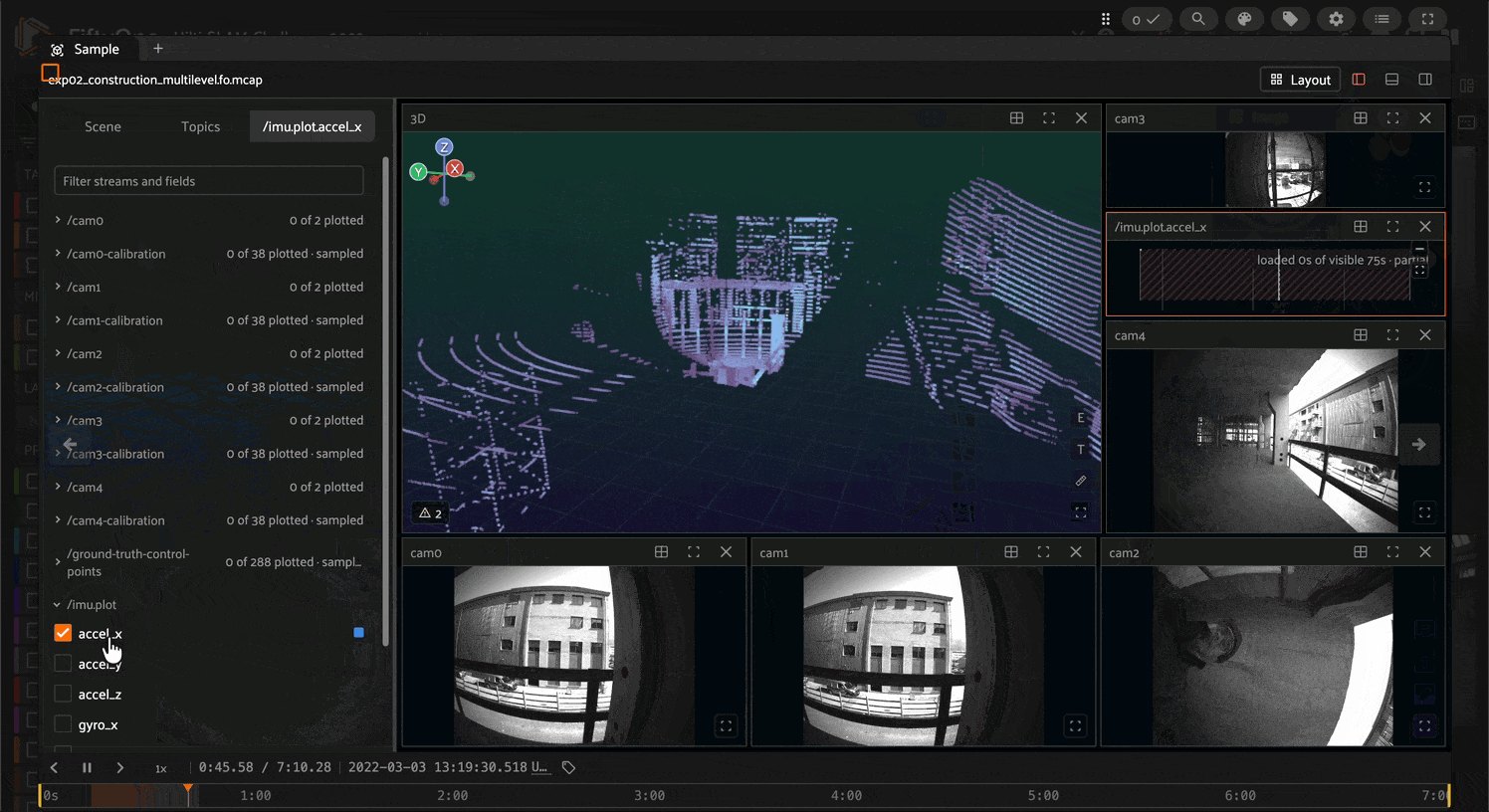
A post went round this week pointing at a Hugging Face Space that opens the Hilti SLAM Challenge data in FiftyOne: scrub the LiDAR and five cameras of a handheld rig through a construction site, in the browser. The pitch was "millimeter-accurate ground truth, in the environments that give SLAM the least to work with", "18 sequences on active construction sites", with "surveyed control points, so precise answers exist where texture doesn't".

That last clause is the interesting part, and it is why I care about this dataset more than most. On a construction site the question is never "does the map look right". It is "is this anchor hole within 10 mm of where the drawing says". Most SLAM benchmarks cannot answer that, because their reference trajectory comes from GNSS-INS (a few centimetres), a motion-capture room (millimetres, but only inside the room), or from registering the LiDAR against a prior map, which fails in the same corridors and stairwells the SLAM system fails in. Hilti's answer is to stop asking another estimator and ask a surveyor.

This piece is about how that ground truth is made, how the score built on it behaves, what won three editions of the challenge, and what the new FiftyOne conversion does and does not carry. I am Satyajit; I build LiDAR pipelines for construction inspection, so I read it as someone who would actually run a system against it.

What is in the box

The Space is a thin wrapper. Its datasets.json loads harpreetsahota/Hilti-SLAM-subset, which holds 5 episodes and 7.08 GB (measured, from the Hub file listing), on a cpu-basic container that clones the dataset per browser, caps at 20 sessions and expires idle clones after 30 minutes (measured, from gateway.py and the README). The full conversion is Voxel51/Hilti-SLAM-Challenge-2022: 18 MCAP episodes, 49.7 GB (measured).

The "18 sequences on active construction sites" line needs two corrections, both from the dataset card and the per-episode records in its samples.json (measured):

It is 16 runs, not 18. One long run, exp23_the_sheldonian_slam, is stored as three bags, so it arrives as three episodes.
Seven runs were recorded at Hilti's construction site in Schaan, Liechtenstein (one of them, exp07, is a 100 m office corridor at Hilti's head office), totalling 25.0 minutes. The other nine were walked through the Sheldonian Theatre in Oxford, a building completed in 1664, totalling 45.7 minutes. The theatre has the narrow stairs, curved surfaces and a cupola; the construction site has the bare concrete.

Across all 18 episodes I count 70.7 minutes, 212,065 camera frames, 42,408 LiDAR sweeps holding 2.55 billion points, 1,692,948 IMU samples and 159 surveyed positions (measured, summed from samples.json; they match the card's own totals). The official release's ground-truth folder has the same 159 sparse rows (measured).

	2021	2022 (the one in FiftyOne)	2023
Platform	Handheld stick	Handheld "Phasma"	Phasma + a 700 kg tracked robot
LiDAR	Ouster OS0-64 + Livox MID70	Hesai PandarXT-32, 10 Hz	PandarXT-32; Robosense Bpearl on the robot
Cameras	5 (Alphasense), 10 Hz	5 fisheye, 720x540, 40 Hz	5 on Phasma; 4 OAK-D stereo pairs on the robot
IMU	ADIS16445, Bosch BMI085, Ouster's	Bosch BMI085, 400 Hz	BMI085; XSens MTi-670 on the robot
Ground truth	Total station (3 mm) or mocap	TLS map + tip on floor crosses	TLS map + tip, or a LiDAR-read floor target
Teams	27	42	69

All of that table is reported, from the three papers (2021, 2022, 2023).

The Phasma handheld rig: a red Alphasense camera head with five cameras on top, a Hesai PandarXT LiDAR below it in a machined aluminium frame with dowel-pinned plates, a handle, and a steel needle tip protruding from the bottom. — Phasma, the 2022 rig: five global-shutter fisheye cameras and the IMU in the red head, a Hesai PandarXT-32 below, and the steel tip at the bottom that is pressed onto each survey mark (Hilti-Oxford paper, Figure 1).

Ground truth, three ways

2021: a total station tracking a prism

The first edition mounted a survey prism on the stick and tracked it with a Hilti PLT 300 robotic total station. Collection was "stop 'n go": the operator stops, the stick is gravity-aligned by a mechanical system, and the station measures the static prism to 3 mm (reported). Indoors in a lab, an optical motion-capture system gave full 6-DoF at under 1 mm and 200 Hz (reported).

The weakness is the one any surveyor knows. A total station needs line of sight. You cannot follow someone down a stairwell into a basement car park with it, and those are exactly the places a construction SLAM system breaks.

2022: a laser-scanned building and a steel tip

The 2022 edition, the one in FiftyOne, inverts the problem. Instead of tracking the device, survey the building first, then bring the device to known points.

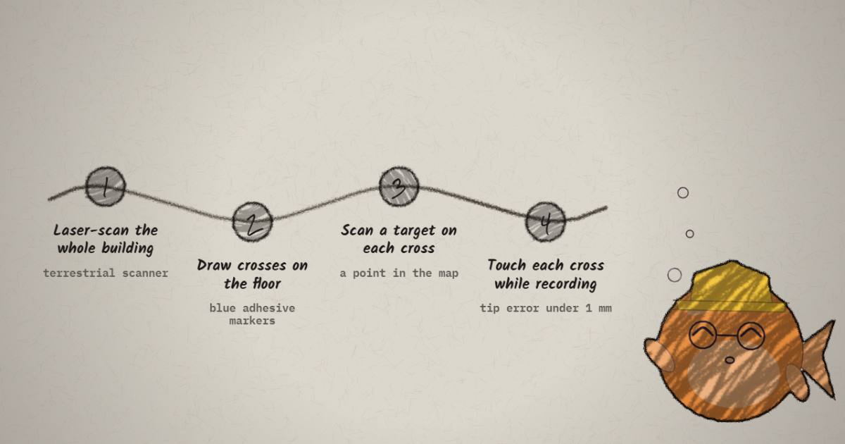
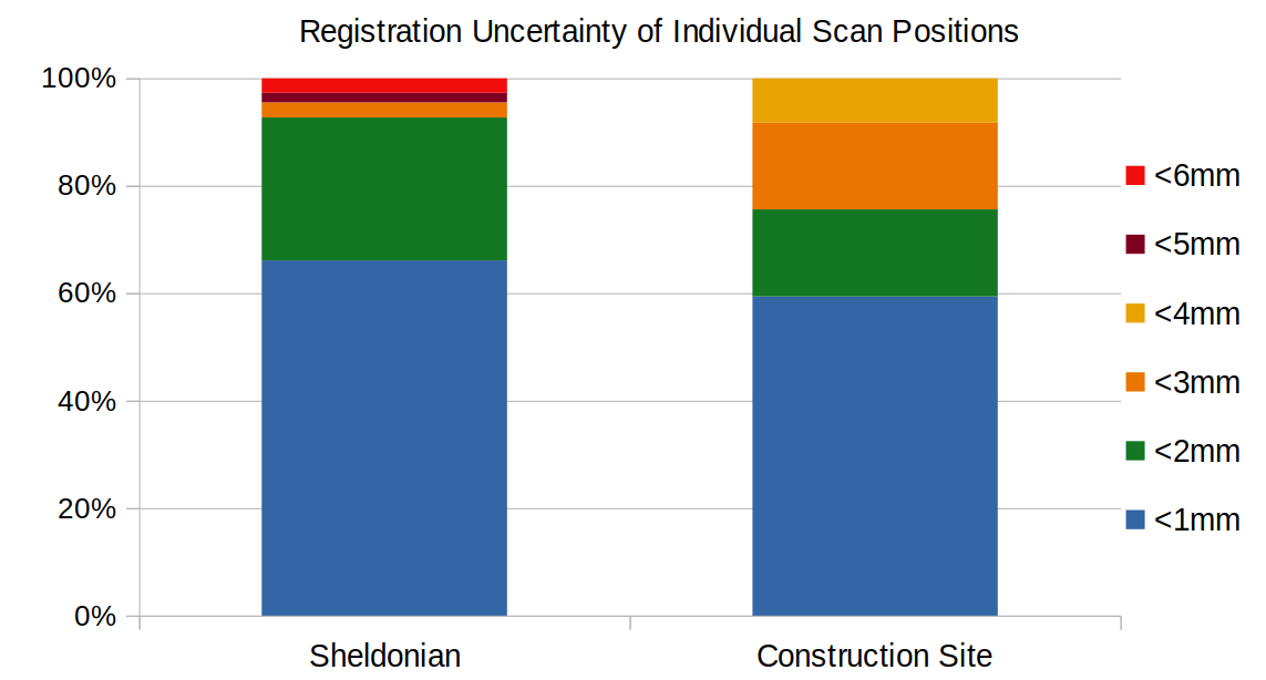
Scan the building. A Z+F Imager 5016 terrestrial laser scanner (TLS) captured both sites: up to 1 million points per second, 360 m range, angular accuracy of 14.4 arcsec (reported). Scans were registered with reflective targets plus plane-to-plane registration and a block adjustment. 91% of Sheldonian scans and 95% of construction-site scans have a position uncertainty within 3 mm (reported, paper Figure 5). The few worse scans are leaf scans with fewer connections, and the authors placed no ground-truth targets in those.
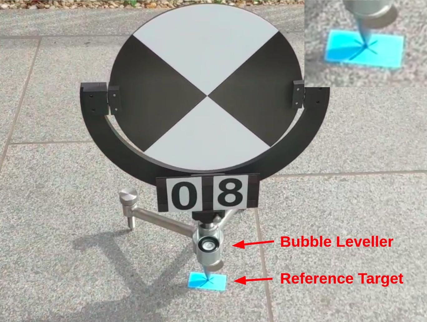
Mark the floor. Draw crosshairs on adhesive blue markers on the floor. Put a levelled checkerboard target's metal tip on each cross, label it, and make sure every target appears in several scans. Each cross is now a point in the registered cloud.
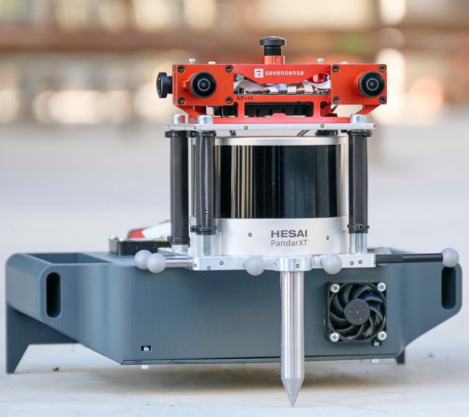
Touch the marks. While recording, the operator stops and places Phasma's steel tip on the cross, taking "several seconds" to keep the manual error under 1 mm (reported). The site was closed and the markers were not moved.

The tip is calibrated against the IMU (the rig was machined, dowel-pinned and checked with a GOM Atos Q3 scanner), so a timestamp at which the device stood on cross P16 is a timestamp at which the IMU sat at a known offset above a point known to a few millimetres. Between marks you know nothing. The paper is explicit that this gives only a handful of instants per run, "between 5 and 10". In the release it ranges from 3 visits (exp18) to 22 (exp02), many of them revisits of the same cross (measured).

A black-and-white checkerboard scanner target on a levelling stand with a bubble leveller, its metal tip resting on a blue adhesive marker with a drawn crosshair on a concrete floor; the target is numbered 08. An inset shows a steel tip touching the blue marker. — A reference target on a floor cross: scanned by the TLS to fix the cross in the map, then removed so the rig's tip can be placed on the same cross during recording (Hilti-Oxford paper, Figure 8).

Stacked bar chart of registration uncertainty of individual scan positions for the Sheldonian and the Construction Site. Most of each bar is under 1 mm and under 2 mm; small slivers reach 3 to 6 mm. — How well the prior map itself is known: registration uncertainty of each TLS scan position relative to the first scan, in millimetre bins (Hilti-Oxford paper, Figure 5).

The same TLS map also gives a second, denser reference. For the "additional" sequences, each deskewed LiDAR scan was registered to the prior map with point-to-point ICP inside the Oxford VILENS estimator, played back slowly. The paper puts that at 1 to 2 cm (reported) and says to use the sparse marks once your system is under 1 cm. I checked that claim below.

2023: a target the robot can read itself

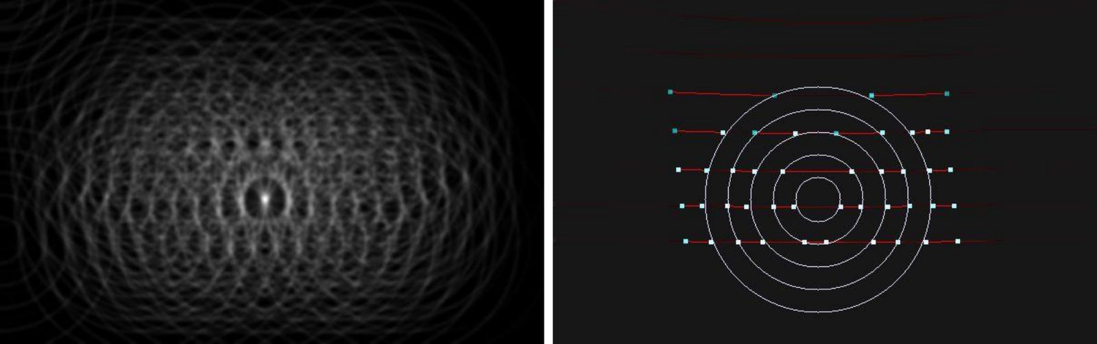
A 700 kg drilling-robot prototype cannot place a needle on a cross to the millimetre. So for 2023 the team designed a floor target the LiDAR can find on its own: a circular pattern on a surveyed point. The detector fits the ground plane, projects several scans onto it, runs a 1-D Canny edge detector along each ring's intensity, and lets every edge vote for circles of the target's known radii in a Hough space. The blurred maximum is the centre, transformed back to 3D.

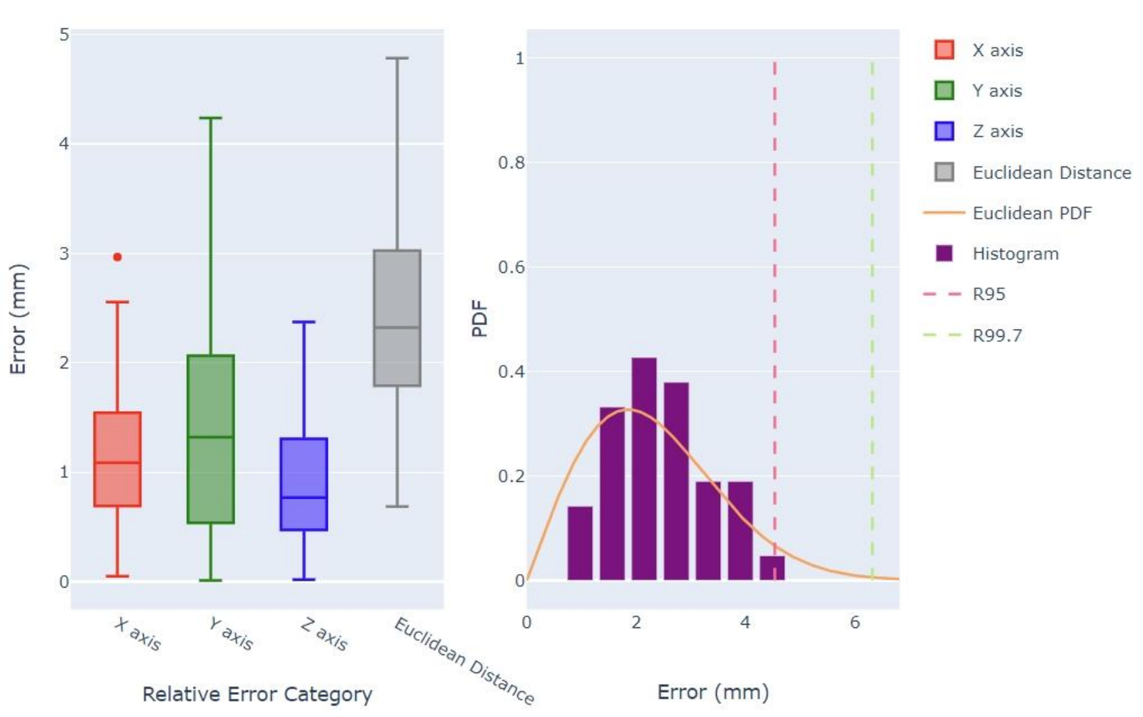
On a pre-surveyed 6x6 test grid the 3-D error has a median of 2.3 mm and a maximum of 4.7 mm; a fitted Rayleigh distribution gives R95 = 4.54 mm (reported, 2023 paper Figure 4). That is relative accuracy between targets on one plane, which the authors say plainly; it does not capture a range-dependent bias of the sensor. A target within 90 cm of the robot is always crossed by at least 3 scan lines (reported). The TLS changed too, to a Trimble X7, mainly because its software registers scans in the field.

Left: a dark circular Hough accumulator with many overlapping rings and a bright peak at the centre. Right: projected LiDAR ring lines with detected intensity edges marked as dots and concentric fitted circles overlaid. — The 2023 ground-control-point detector: votes from intensity edges along each LiDAR ring accumulate in a circular Hough space (left); the peak gives the target centre, shown with the fitted circles over the detected edges (right) (Hilti 2023 paper, Figure 3a and 3b).

Left: box plots of relative error per axis and Euclidean distance, all under about 5 mm. Right: histogram of 3-DoF Euclidean error with a fitted Rayleigh curve and R95 and R99.7 markers near 4.5 and 6.3 mm. — Accuracy of the LiDAR-read targets on a surveyed grid: per-axis and Euclidean error, and a Rayleigh fit to the Euclidean error with its R95 and R99.7 lines (Hilti 2023 paper, Figure 4).

The score, and why it is not RMSE

Every edition scores a submission per survey visit, not per pose. The 2022 procedure, from the paper and the official evaluation.py:

Transform each estimated IMU pose to the pole tip with a fixed offset. In the script it is a pure translation of (0.059, -0.00855, 0.1964) m in the IMU frame, applied to every sparse reference file.
Associate estimate and reference by timestamp (evo, up to 2 s apart) and align them with a rigid SE(3) Umeyama fit, no scale.
Score each mark by its absolute distance error $e_i$ , and normalise per sequence.

s_i = \begin{cases} 10 & e_i \lt 1\,\text{cm} \\ 6 & 1 \le e_i \lt 3\,\text{cm} \\ 3 & 3 \le e_i \lt 6\,\text{cm} \\ 1 & 6 \le e_i \lt 10\,\text{cm} \\ 0 & e_i \ge 10\,\text{cm} \end{cases} \qquad S_j = \frac{100}{10N}\sum_{i=1}^{N} s_i

$N$ is the number of marks in sequence $j$ , so every sequence is worth 100 and the final score is the sum. Eight challenge sequences make 800 the ceiling (reasoned). 2023 added a top band (20 points under 5 mm) and a tail band (1 point from 10 to 40 cm), and normalises by $20N$ .

Three properties fall out of that, and each matters if you tune against it.

It is a staircase. A mark at 9 mm earns 10 points; at 11 mm, 6. Nothing rewards going from 11 mm to 29 mm. RMSE is smooth; this is not.
Missing marks score zero instead of exploding. That was the stated reason for the design in 2021: incomplete trajectories can still be ranked. It also means a team can rank above one with a lower RMSE. The 2022 paper names KTH and NTU: better mean ATE, lower score, because most of their errors sat just above the 3 cm edge.
Only position at a few instants is scored. Orientation never enters, and neither does anything between marks. A system can wander between crosses as long as it is back on them.

The widget below makes the staircase concrete on real geometry: the 13 visits of exp01, read from the official ground-truth file. The trajectory is simulated: heading drift that grows with distance walked between marks, plus a fixed noise pattern, then a rigid fit in the plane.

exp01 construction ground level, 13 survey visits

76.2/ 100 for this sequence

RMSE 16 mm · worst visit 32 mm · 130 m between marks

heading drift0.10° / 100 mper-visit noise (1σ)3 mm

error per visit, in visit order (dashed: band edges)

0–10 mm: 10 pts × 610–30 mm: 6 pts × 630–60 mm: 3 pts × 160–100 mm: 1 pts × 0≥ 100 mm: 0 pts × 0

The marks are real; the trajectory is simulated. Heading drift accumulates over the straight-line distance between consecutive marks, which understates the path actually walked. Alignment is a rigid fit in the plane, the 2D case of the challenge's SE(3) Umeyama step.

What it shows, with the numbers computed by the same model in Python (reasoned):

Noise alone is free in 2022 and expensive in 2023. With 5 mm of per-visit noise and no drift, the RMSE is 6.1 mm and the 2022 score is a perfect 100; the 2023 bands give 65.4, because most visits fall out of the under-5 mm band. At 8 mm of noise it is 84.6 and 46.2.
A tenth of a degree per 100 m is a quarter of the score. With 0.1° of heading drift per 100 m and 3 mm of noise, the RMSE is 15.7 mm and the 2022 score falls to 76.2. The worst visit is the last one, back on P13: 31.5 mm. Drift that a loop closure would remove shows up exactly where the run returns to its start. At 0.25° per 100 m the score is 52.3.
Alignment hides part of the drift. The rigid fit spreads the error over the whole loop, so the middle visits (P19, P31, P32) stay under 10 mm even at 0.25° per 100 m. The paper notes the matching effect of loop closures, which sometimes "distributed the error from one particular section to the whole trajectory".

The straight-line distance between exp01's marks is 130 m (measured), a lower bound on what the operator walked.

What won, and what that says

Year	Winner	Method	Score	Note
2021	Megvii	a FAST-LIO2 variant, Ouster + Livox fused	461	mean error 9.3 cm on all sequences
2022	CSIRO	Wildcat SLAM, continuous-time LIO + offline global optimisation	563.8 of 800	mean RMSE ATE 2.07 cm
2022, 3rd	HKU MaRS	FAST-LIO2 + BALM	400.4
2023	KAIST URL	AdaLIO front end, Quatro loop closure, factor graph	1177.64	100% mark coverage

All reported, from the papers' leaderboards. The pattern for a LiDAR person is blunt. In 2021 the first four places were commercial, all LiDAR plus IMU. In 2022 the top four used no camera at all; of the top 25, all used LiDAR and IMU, only 10 used cameras; the best vision-only system (OKVIS2.0) scored 32.5 with typical errors of 10 to 20 cm. In 2023 FT-LVIO was the only camera-augmented LiDAR system in the top ten. FAST-LIO2 runs through all three editions: the 2021 winner, the 2022 third place, a base for several 2022 entries, and the LiDAR odometry inside ETH's 2023 multi-session winner. If you want the filter itself, I derived it in FAST-LIO2 from scratch.

The per-sequence errors of the 2022 top three are more useful than the totals (reported, RMSE ATE in cm, paper Figure 9):

Team	Exp11	Exp01	Exp02	Exp21	Exp03	Exp07	Exp15	Exp09
CSIRO	0.9	1.0	1.9	1.5	0.9	3.7	2.7	4.0
Vision & Robotics	0.7	1.1	2.0	1.1	4.8	5.1	6.6	10.1
HKU	0.9	1.0	2.0	5.1	2.1	4.6	13.9	17.8

Open floors with overlap are solved to about a centimetre. The long corridor (exp07, failing around 46 s in) and the Sheldonian stairs (exp09 from 132 s, exp15) are not. HKU's FAST-LIO2 pipeline matches the winner on the open sequences and loses an order of magnitude in the narrow stairs.

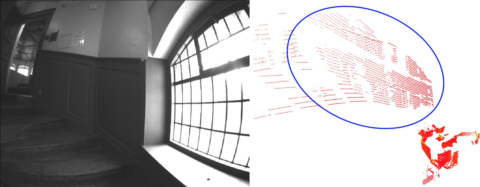
Why did the cameras not matter, in a dataset designed to make them matter? The authors' own answer: the PandarXT-32's range and accuracy (±1 cm, reported) kept finding geometry. In a narrow Sheldonian staircase it saw out through small windows to the next building and the ground; with an operator walking in front, it still caught the slanted ceiling and the rails.

Left: a fisheye camera frame inside a narrow wood-panelled staircase with a tall window. Right: the matching LiDAR scan in red, with a blue ellipse around points that lie outside the building, seen through the window. — Why LiDAR-inertial systems survived the 'degenerate' stairs: inside a narrow Sheldonian staircase the LiDAR scans the adjacent building and the ground through a window (circled), which constrains the estimate (Hilti-Oxford paper, Figure 10, left).

Two more details from the 2023 paper are worth knowing before you trust any live leaderboard. Teams found they could recover the mark coordinates from the error plots the submission server returned, and hand-edit trajectories near the mark timestamps; the organisers detected this, removed submissions, and added a third site with no feedback plots and double weight. And in the 2023 multi-session track only two teams per modality had entered when the paper was written.

I scored the dense reference against the marks

The paper says the dense, ICP-to-map reference is good to 1 to 2 cm. Six sequences have both references: exp04, exp05 and exp06 (dense files in the challenge's GitHub repo) and exp14, exp16 and exp18 (on the Hugging Face release). So I treated each dense trajectory as if it were a submission and scored it the official way: tip offset from evaluation.py, the pose interpolated at each mark's timestamp (the rig is stationary there; I checked the dense speed is at most 0.03 m/s at every mark), SE(3) Umeyama, per-mark error (measured):

Sequence	Marks used	RMSE (mm)	Worst (mm)	Without the tip offset (mm)
exp14 basement 2	4	6.7	10.0	61.6
exp05 upper level 2	6	19.9	33.0	56.0
exp06 upper level 3	7	23.3	36.4	68.0
exp04 upper level	7	29.4	59.3	59.6
exp16 attic to upper gallery 2	9	76.0	160.6	80.0

exp18 has two marks inside the dense span, too few for a rotation, and a translation-only fit leaves both at 155.1 mm (measured). Before alignment the sparse marks also sit about 0.3 m above the tip-corrected dense poses on every sequence; the rigid fit absorbs that constant.

Three readings, the first two measured and the third reasoned:

On the construction-site runs the dense reference agrees with the marks at about 2 to 3 cm RMSE, slightly worse than the paper's 1 to 2 cm. In the Sheldonian attic run it is 7.6 cm, with one mark at 16 cm. That is the same range as CSIRO's 2.07 cm mean, which is the point: at the top of the leaderboard the dense reference is no longer a referee.
Forget the tip and you add 3 to 5 cm to the construction runs. If you score your own system against the sparse positions in the MCAP, apply the same offset the evaluator does.
So use the dense trajectory to find where your odometry broke, as the authors intended, and the marks to say how well it did. A dense "ground truth" from scan-to-map ICP inherits the degeneracies of scan-to-map ICP.

The FiftyOne conversion: what MCAP buys and what it drops

The conversion turns each ROS 1 bag into an MCAP file whose channels FiftyOne and Foxglove can show together. I read the summary section of exp14_basement_2.fo.mcap with HTTP range requests (the file is 844 MB; the summary is 134 KB at the end) and listed its channels (measured): 17 channels, 35,372 messages in 741 chunks. Cameras are foxglove.CompressedImage, LiDAR is foxglove.PointCloud, the frame tree is foxglove.FrameTransform, the dense reference is foxglove.PoseInFrame, all protobuf. The IMU is different: /imu.plot is a JSON channel with a custom PlotScalars schema, 29,539 messages for 74 s. It is built to be plotted, not consumed by an estimator.

The FiftyOne app showing exp02_construction_multilevel.fo.mcap: a 3D LiDAR point cloud panel, five fisheye camera panels of a building under construction, an IMU acceleration plot, a channel list on the left, and a timeline at the bottom reading 0:45.58 of 7:10.28. — One episode in FiftyOne: the LiDAR sweep in 3D, five synchronised fisheye cameras, and an IMU channel plotted on the same timeline (Voxel51 Hilti-SLAM-Challenge-2022 dataset card animation).

What changed, from the card, and what it costs:

Cameras at 10 Hz, not 40, as JPEG quality 92 instead of raw 8-bit greyscale. Fine for looking. Not the data a visual-inertial system was tuned on.
LiDAR per-point time rebased to an offset from the sweep start. This one is a fix. A float32 near 1.65e9 s has a spacing of 128 s (reasoned: $2^{30} \le 1.65\times10^9 \lt 2^{31}$ , so the spacing is $2^{30-23}$ ), which would make every point in a sweep share one timestamp and break deskewing.
No TLS scans, CAD or calibration reports. The .e57 laser scans, the map you would localise against, are only in the original release.
Size. The original rosbags total 336 GB; the MCAP set is 49.7 GB, about 6.8x smaller (measured from both Hub listings; reasoned ratio). Most of that is the camera rate and JPEG.

Two small inconsistencies in the sources, both measured against the files: the paper lists Exp09 as 367 s and Exp10 as 446 s, but exp09's marks alone span 439.9 s and its episode is 446.6 s, while exp10's is 370.3 s; the two durations are swapped in the paper. And exp23's three bags hold 974 s of recording for a run whose marks span 1,049 s, so there are gaps between the parts.

If you plan to evaluate a system, use the original bags and evaluation.py; if you want to see where a run goes wrong before you download 30 GB, the FiftyOne episodes are good for that. I have not run the Space interactively at scale; its 20-session cap suggests it is a demo, not a workbench.

Hilti-Research/hilti-slam-challenge-2022@e4aacf7 · snapshot 2026-10-06

tracked files

branch: main
tests: none found
source: 25.1 kB
commit date: 2026-08-10

source by language

Python25.1 kB(2)

by size of tracked source at this commit, file counts in brackets; docs, data and vendored trees excluded

local clone, 2026-10-06 at e4aacf7 — branch, commit, commitDate, fileCount, hasTests, languages, shallow

shallow clone: counts describe the pinned tree, not the history

The licence

All three editions are published under CC BY-NC-SA 3.0 (reported, from the challenge site and both Hub cards): attribution, no commercial use, and derivatives under the same licence. The Voxel51 conversion carries the same terms. For anyone in industry, that is the line to read twice: benchmarking a commercial product on this data is a question for Hilti (challenge@hilti.com), not something the licence grants.

Honest notes

Sparse truth sees a few instants. 159 positions over 70.7 minutes is one every 27 s on average (reasoned). It certifies where you were at a cross, not your map, not your orientation, and not the stretch between crosses where most drift lives.
The rig stops at every mark. Each visit is a few seconds standing still on a needle. A zero-velocity update falls out of that for free, which a real walking survey would not give you.
The extrinsics are not fully external. The 2022 paper admits there was no separate LiDAR-to-IMU calibration and that this "may have resulted in a few millimeters of error in the ground truth control points". The 2023 edition let teams submit their own extrinsics; none of the top teams did.
What I did not verify. I did not download a bag or run any SLAM system; the per-sequence errors and scores above are the papers'. My dense-versus-sparse numbers depend on reading the dense files as IMU poses in x y z qx qy qz qw order and on the tip offset in evaluation.py; the unexplained 0.3 m vertical offset makes me less than certain the frames are what the filenames say.

For the related capture side of the same sites (how people get from a walk-through to a scene you can measure), see Gaussian-splat capture in practice; for the back end most of these winners share, GTSAM 4.3; and for LiDAR-inertial odometry at the opposite end of the speed range, FAR-LIO.