2026-09-26 · 23 min · 3d · gaussian-splatting · vision-language-models · benchmarks · paper · explainer

Six 3D papers crossed my feed in the last week of September 2026, each as a one-line claim. Surpasses GPT6 Astra. Higher PSNR than 3DGS at a quarter of the size. Significant gains in boundary mIoU. Better spatial reasoning. They attack four problems, so I have grouped them by problem. For each I read the paper, the project page and any released code, and asked: what problem, what one idea, what evidence against which baselines, and what can you run.
| Item | Problem | The one idea | Headline, and what it is measured on | Released |
|---|---|---|---|---|
| Mira-Scene | Room from one photo | Predict each pixel's canonical object coordinate; solve the pose | 3D-IoU 0.520 → 0.727 over SAM 3D on BlendSwap. "Beats GPT-6 Astra": six viewers, no metric | Code (no licence file), checkpoints, eval set |
| HARMONY | Room from one photo | A VLM places objects in order; geometry corrects them | Best on all six metrics over 100 Front3D renders, GPT-6 Astra included | Code (MIT), benchmark |
| DAVINCI | Floaters on shiny objects | Mesh, Voronoi albedo, separate specular term | Mean PSNR −0.08 dB vs 3DGS at 4.0× smaller; +1.58 to +3.26 dB on the four reflective scenes | Preprint (CC BY 4.0), no code |
| D3GS | Floaters from few views | Metric depth, DINO features, diffusion refinement | Best or near-best on three datasets; +0.03 dB on LLFF 3-view, +2.40 dB on Mip-NeRF 360 3-view | Nothing found |
| NG-GS | Ragged object edges | A small NeRF smooths boundary Gaussians | Boundary mIoU +4.4 to +6.8 points over COB-GS; mIoU +0.5 to +2.7 | Code, non-commercial |
| Imagine3D-LLM | 3D questions from photos | The MLLM decodes Gaussians from summary tokens while training | +7.3 SQA3D, +7.6 SPAR-Bench over its own same-data baseline | Paper PDF; code "coming soon" |
The background, once
Gaussian splatting in one paragraph
A 3D Gaussian Splatting (3DGS) scene is a cloud of anisotropic 3D Gaussians, each with a mean, a covariance (a rotation and three scales, so it can be a ball, a disc or a needle), an opacity, and a colour that varies with viewing direction through low-order spherical harmonics. A pixel sorts the Gaussians covering it by depth and composites them front to back:
where is opacity times the Gaussian's projected footprint at the pixel and is the transmittance left when the ray reaches it. Training starts from a structure-from-motion point cloud and densifies as it goes, cloning or splitting Gaussians whose position gradient stays large and pruning those whose opacity collapses. Nothing in it says a Gaussian must sit on a surface. (For the whole pipeline in one program, see Spirula Studio.)
Why a reflection becomes a floater
A reflection is not attached to the surface that shows it: move your head and the highlight slides across the chrome. 3DGS has two ways to represent that. The honest one is view-dependent colour on the surface, but third-degree spherical harmonics are too smooth in direction to make a spike that is bright over a few degrees and dark elsewhere. The other is matter: a bright, semi-transparent Gaussian somewhere on the rays that saw the highlight. One image cannot tell depth along its own rays, so the optimiser can hang it anywhere on them and match the photo. From every other view it is in the wrong place. A floater is not noise; it is a highlight stored at the wrong depth.
The toy below is that argument in 2D: a flat, slightly shiny surface of seven flattened Gaussians, a light overhead, and a 64-pixel camera on an arc, each pixel composited with the equation above. The true image adds a reflection read at the surface along the mirror direction. Splats + floater keeps the surface colour view-independent and adds one bright Gaussian on the 0° camera's ray, its width and opacity grid-searched to match the 0° view and nothing else. Splats + specular term adds a reflection lobe read along the mirror direction instead, deliberately the wrong width (κ 45 where the truth is 60), standing in for a learned one.
In the toy (measured, in the toy only), the floater fit scores 33.7 dB PSNR at 0°, 13.8 dB at ±10° and 10.0 dB at ±40°. Drawing no highlight at all scores 15.3 to 16.2 dB, so away from its fit view the floater is worse than leaving the highlight out: it pays where the highlight should be and again where it wrongly is. It even moves the wrong way. At +20° the real reflection shifts to +x; the floater, nearer the camera than the surface, lands at −x. The specular term, wrong width and all, holds 35.1 to 36.0 dB at every angle because it is evaluated where the reflection happens. The per-ray table is the compositing sum written out for the brightest pixel.
Few input views make this worse: fewer rays pin depth, and any disagreement between photos, including a lighting change, is cheaper to explain with extra matter than with the right colour.
Single-image 3D, and why placement is the hard part
Object-level image-to-3D (TRELLIS, Hunyuan3D, SAM 3D) now turns one crop into a good asset, but in a canonical frame: centred, normalised, upright. A room from one photo also needs each object's scale, rotation and translation in the camera frame, under occlusion, with unknown depth scale. Holistic methods generate the scene as one asset, so every object competes for one token budget and small things come out mushy. Compositional methods generate objects separately and then place them. Placement is the open part, and both papers in the first group are about it.
A room from one photo
Mira-Scene: predict coordinates, then solve the pose
Problem. Compositional methods usually regress each object's pose: seven numbers, sparse and unbounded, hard to learn from the little scene-level 3D data there is.
The idea. Predict something dense and bounded instead. For each visible pixel of an object, the model predicts a Canonical Coordinate Map (CCM): which point of the object's normalised shape that pixel shows, as an in a unit cube. Monocular depth gives a Point Cloud Map (PCM): where the pixel is in the scene. Every pixel is now a correspondence, and the pose is the similarity transform that best maps one set onto the other, found by RANSAC and solved in closed form with Umeyama's algorithm. Because CCM lives in the object's own frame, it can be trained on renders of isolated objects with no scene layouts at all. A Mixture-of-Transformers generates the object's voxels and its CCM together, as two expert streams sharing self-attention.
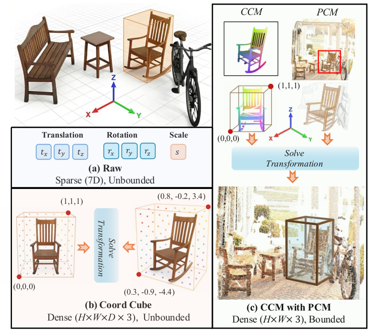
The evidence (reported). On BlendSwap, with every method given the same image and ground-truth instance masks:
| BlendSwap | CD ↓ | F@0.1 ↑ | EMD ↓ | 3D-IoU ↑ | ICP-Rot ↓ | 2D-IoU ↑ | ADD-S ↓ |
|---|---|---|---|---|---|---|---|
| SAM 3D | 0.027 | 0.817 | 0.163 | 0.520 | 7.566 | 0.672 | 0.078 |
| Mira-Scene | 0.021 | 0.843 | 0.169 | 0.727 | 5.616 | 0.783 | 0.031 |
The abstract's "relative gains of 39.8% in 3D-IoU and 16.5% in 2D-IoU" are these columns. On 50 examples the authors selected from 3D-Future Scene the layout gain is smaller (3D-IoU 0.596 → 0.694), and SAM 3D keeps the better geometry (CD 0.014 against 0.015). The released BlendSwap set holds 15 scenes, per its dataset card.
Three caveats. The ablation mixes two effects: the representation swap takes 3D-IoU from 0.379 to 0.727, but with matched training data CCM reaches 0.537, and the rest is object-level data only CCM can use (reasoned). The geometry expert predicts only voxels; the scored meshes come from SAM 3D's own second-stage mesh module. And the numbers use ground-truth masks; the GPT-5.6-driven automatic segmentation is for demos.
What "surpasses GPT-6 Astra" is measured on
The launch post said Mira-Scene "surpasses GPT6 Astra in terms of geometric detail and reconstruction consistency". The paper never mentions Astra. The claim lives on the project page, in a section titled "Compared to GPT-6 Astra From Scratch": six cases, each a pair of 3D viewers. Left is a scene "built from scratch by GPT-6 Astra"; right is "a Mira-Scene reconstruction with Astra for building background". The verdict is one sentence, "Mira-Scene delivers stronger image consistency", with no metric and no protocol, and Astra is on both sides. Six scenes you can orbit and judge yourself is more than many claims offer, but it is not a measurement. For an Astra number, see the next paper.
HARMONY: let the VLM place, let geometry correct
Problem. The same placement problem from the other side. A VLM knows the sofa's back is against the left wall but cannot place it to a centimetre; a point-map model places precisely but knows nothing about what leans on what.
The idea. Use both, in a fixed order. A VLM guesses the room's size and picks the deepest visible corner; VGGT's point cloud gives a Manhattan frame that calibrates the camera to that corner. Each object is segmented, inpainted and lifted to a mesh with Hunyuan3D. Placement goes wall-mounted items, then furniture depth-first outward from the corner, so each new piece lands in front of everything placed, then decorations on their hosts. The VLM sets relations and yaw; the silhouette then fixes lateral position and the scale-to-depth ratio, and the point cloud fixes depth. After each stage the VLM compares a render with the photo and corrects what it finds.
The evidence (reported), on 100 Front3D renders:
| Front3D, 100 images | N-CLIP ↓ | PL ↓ | CD ↓ | F@0.1 ↑ |
|---|---|---|---|---|
| Best other baseline | 0.127 (SAM 3D) | 0.043 (Gen3DSR) | 0.052 (CAST) | 85.70 (CAST) |
| GPT-6 Astra | 0.095 | 0.052 | 0.061 | 77.44 |
| HARMONY | 0.092 | 0.041 | 0.049 | 89.82 |
On 30 real photos it scores N-CLIP 0.112 against Astra's 0.127; in a 16-person user study over 20 scenes, without Astra, it ranked first in 67.0% of choices. N-CLIP, one minus the CLIP similarity of render and photo, barely separates HARMONY from Astra; the geometry does, F-score 89.82 against 77.44, matching the paper's line that Astra "exhibits larger geometric errors, e.g., beds might not align with walls." The abstract calls the Astra comparison "qualitative" despite the Astra rows, and nothing says how Astra was prompted. Nor does the paper name its own VLM; the code defaults to a local Qwen3-VL-30B-A3B. Its failure section is candid: 25.9% of detections carry low grounding confidence.
The two papers share no benchmark or metric, so nothing ranks them against each other. Both beat SAM 3D on their own ground.
Floaters: shiny objects and few photos
DAVINCI: take the reflection out of the Gaussians
The post credited Killian Rando and said the source was in the replies. It is: the reply links Rando's announcement, which links a HAL preprint, Deferred Anisotropic Voronoi Inversion with NASGabor Captured Illumination, by Rando and Jérémie Le Garrec of CEA-List, posted 22 September 2026.
Problem. The toy's: on reflective objects, 3DGS explains highlights with floating matter.
The idea. Drop the Gaussians and give the reflection its own term. From calibrated views and a mesh, DAVINCI learns two terms that meet only in the final image. The albedo is a differentiable anisotropic Voronoi diagram in the mesh's UV space: each site carries ten numbers (position, colour, a temperature for edge sharpness, radius, anisotropy), each texel blends its eight nearest sites, and every 1,000 iterations the 5% least useful sites are pruned and the 5% pulled hardest are split. The reflection is read along the mirror direction from 1,024 learned light probes of four NASGabor lobes each (an angular envelope times a cosine carrier, so one lobe can hold structure rather than a blob), blended with a learned cube map for the far field. One photometric loss trains everything, with no material supervision.
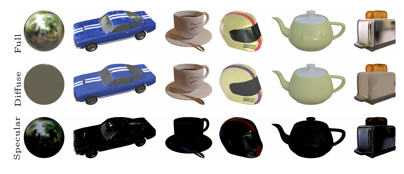
The evidence (reported): Ref-NeRF's six glossy scenes, 200 test views each, 30,000 iterations on both sides, against the official 3DGS on an H100.
| Scene | 3DGS PSNR | DAVINCI PSNR | Δ | 3DGS MB | DAVINCI MB |
|---|---|---|---|---|---|
| ball | 27.76 | 30.23 | +2.47 | 18.1 | 12.9 |
| car | 27.22 | 28.80 | +1.58 | 69.8 | 13.1 |
| helmet | 28.42 | 30.69 | +2.27 | 25.9 | 9.8 |
| toaster | 20.93 | 24.19 | +3.26 | 78.8 | 9.1 |
| coffee | 32.27 | 26.89 | −5.38 | 34.4 | 6.6 |
| teapot | 45.80 | 41.14 | −4.66 | 8.6 | 6.7 |
| mean | 30.40 | 30.32 | −0.08 | 39.2 | 9.7 |
The authors measured their own run-to-run noise (0.21 dB on car, 0.25 dB on toaster) and say the mean alone "says nothing". The split is the result: +1.58 to +3.26 dB on the four view-dependent scenes, about 5 dB worse on the two matte ones, where free Gaussians beat an albedo pinned to a surface. LPIPS favours 3DGS on average (0.0829 against 0.0914).
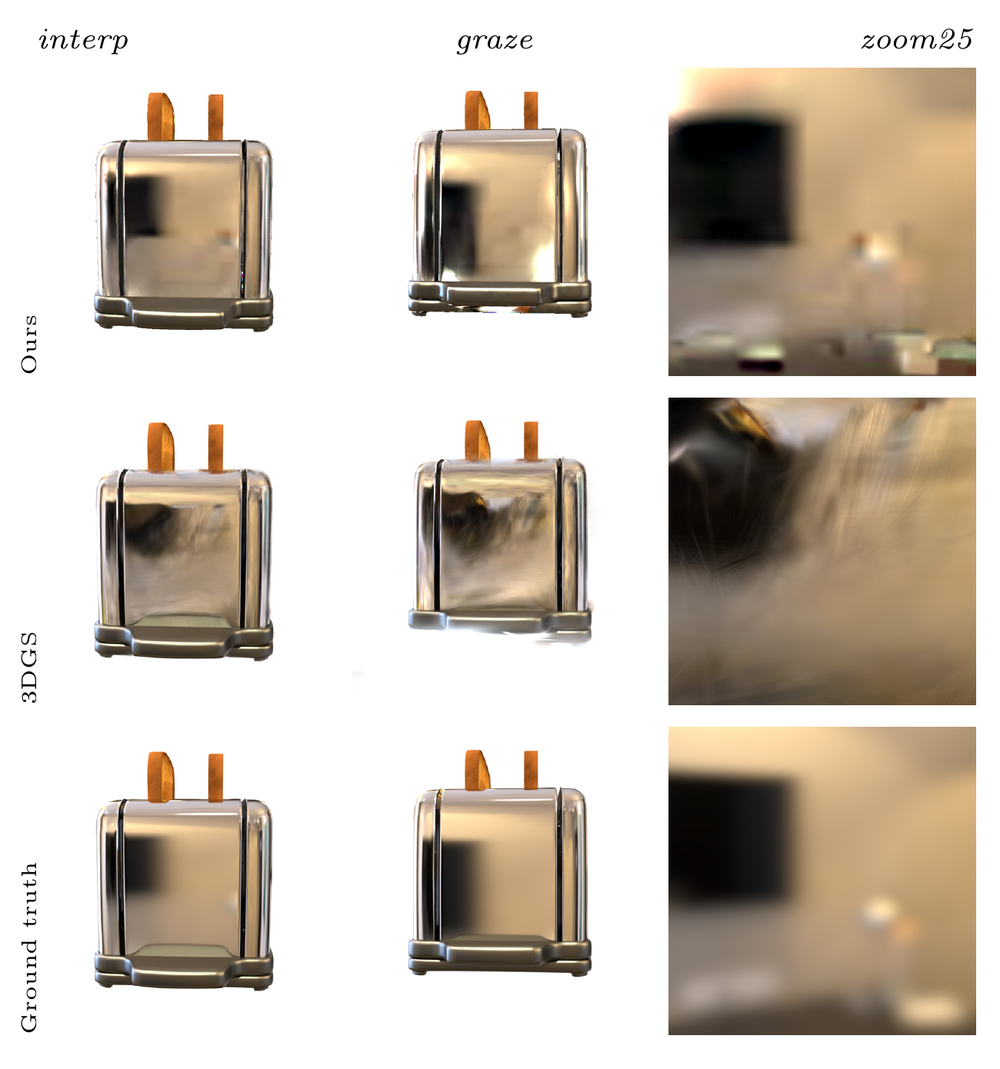
Away from the training poses the gap grows: the published test split lies inside the training cameras' range, so the authors re-rendered harder regimes, and on toaster the gain goes from +2.69 dB to +4.61 dB at the closest zoom. The one loss is car at grazing angles, by 0.30 dB.
Is "a quarter the size" at equal quality? On average, yes: 9.7 MB against 39.2 MB, 4.0×, at a mean PSNR 0.08 dB lower, inside the noise. Per scene it is two stories: on the four reflective scenes DAVINCI is smaller (1.4× on ball to 8.7× on toaster) and better; on coffee it is 5.2× smaller and 5.38 dB worse. And the sizes count the mesh, but the mesh is an input. The paper does not say where its Ref-NeRF meshes came from, and its limitations say the method "assumes a mesh is provided, which does not exist for a real capture", since meshing a reflective object from photos is where geometry "tends to follow the reflection rather than the surface". 3DGS found its geometry from the photos; DAVINCI was handed it.
"Real-time" is plausible, since everything is rasterised, but no frame rate is reported, and training takes 16 to 34 minutes a scene against 6 to 11. The decomposition check flags only a diffuse term brighter than the photo; on the chrome ball the ratio is 0.79, so a mirror's "albedo" carries most of its light (reasoned from their Table 7). The appendix gives the full configuration "should the code not be available"; I found no code.
D3GS: three priors for three failure modes
Problem. Novel views from 3, 6 or 9 photos, where floaters come from ambiguous depth, photos that disagree (the same tabletop under different light), and regions no photo saw.
The idea. One prior per cause. Depth: MapAnything poses and points, refined by bundle adjustment, projected to sparse depth, completed by a diffusion U-Net and sharpened by a DPT decoder, in metric units; it initialises the Gaussians and constrains their depth. Consistency: each Gaussian carries a three-number feature, composited like colour and matched to DINO features reduced to three dimensions by PCA. DINO stays stable across views when RGB does not, so a lighting change stops being explained by extra matter. Unseen regions: a single-step diffusion model, fine-tuned on SynCamMaster, repairs novel-view renders, fed back over several rounds.
The evidence (reported), against PGSR, DNGaussian, FSGS, CoR-GS, DropGaussian, BinocularGS, AnySplat and Difix3D+, plus GenFusion on Mip-NeRF 360:
| PSNR (dB) | D3GS | Best other |
|---|---|---|
| LLFF, 3 views | 21.47 | 21.44 (BinocularGS) |
| DTU, 6 views | 26.04 | 24.51 (CoR-GS) |
| DTU, 9 views | 27.16 | 27.18 (CoR-GS) |
| Mip-NeRF 360, 3 views | 17.69 | 15.29 (GenFusion) |
The margins are uneven: 0.03 dB on LLFF with three views (the LPIPS win, 0.131 against 0.168, is clearer), a 0.02 dB loss on DTU with nine, which the paper states, and +2.40 dB on Mip-NeRF 360 with three. The subset ablation shows the priors add up: 16.89 dB with none to 20.75 dB with all three on DTU. One caution, reasoned: a diffusion prior scored by PSNR against held-out photos is rewarded for agreeing with them, not for being right about what no photo saw. About 25 minutes a scene on an RTX 3090. No code is linked or findable. The "fine on input views, wrong elsewhere" pattern is the one VoxelTTO is built around.
Labels on splats: NG-GS
Problem. Segment an object in a trained 3DGS scene and its edge comes out ragged: a Gaussian straddling the boundary belongs half to each side. Carveout met the same question for a whole scene and answered with FlashSplat's contribution-weighted vote; NG-GS counts FlashSplat among its baselines.
The idea. Make the edge continuous. NG-GS flags boundary Gaussians by the variance of their per-view mask signals, samples rays through the boundary with eight points each, interpolates a feature at each point from nearby Gaussians with radial basis functions, adds a multi-resolution hash encoding, and feeds both to a small NeRF. Losses tie the NeRF's and the splats' colour and opacity together at the boundary, and weight the mask loss by the NeRF's density. The 2D teacher is not quite what the post said: the paper's figure says "SAM2+DINO", and the repository makes that Grounded-SAM-2, where Grounding DINO turns a text prompt into boxes for SAM 2. DINO is a detector here, not a feature teacher.
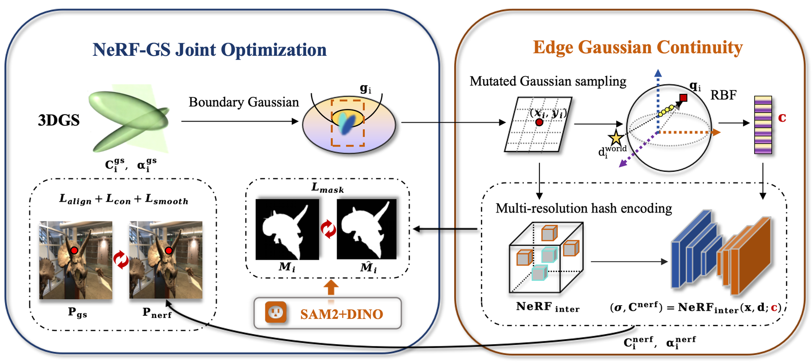
The evidence (reported), in percent:
| Benchmark | Boundary mIoU, COB-GS → NG-GS | mIoU, COB-GS → NG-GS |
|---|---|---|
| NVOS (8 scenes) | 79.1 → 84.7 | 92.1 → 92.6 |
| LERF-OVS (3 scenes) | 68.4 → 72.8 | 82.4 → 82.9 |
| ScanNet | 52.8 → 59.6 | 61.6 → 64.3 |
The "significant gains" are 5.6, 4.4 and 6.8 points of boundary mIoU; plain mIoU moves 0.5, 0.5 and 2.7. Boundary mIoU is the right metric for a boundary method, on a small base: NVOS and LERF-OVS are 11 scenes together. In the ablation, the RBF, hash encoding and NeRF together are worth 2.9 points of boundary mIoU on NVOS (reasoned from their Table 5).
Two inconsistencies. Table 6, labelled as the fortress scene, reports exactly the method's eight-scene NVOS average, 92.6 and 84.7. And τ = 0.6 is defined as a cut on the variance of mask values in [0, 1], which cannot exceed 0.25, so as written the boundary set is empty (reasoned).
What is released (measured, by reading, not running). At commit
7afa887 the boundary module is scene/ngs_model.py, 166 lines. It picks up
to 4,096 Gaussians, ranked mainly by of their mask probability ,
not by variance. It runs a small MLP on hash-encoded Gaussian centres
(nearest-cell lookup, not Instant-NGP's interpolation) with no rays, no
sample points and no volume rendering; density enters only as a regulariser
of weight 0.001. The mask loss is a plain inside-minus-outside sum, not the
paper's density-weighted cross-entropy, and the NG-GS term is added only in
the colour phase of training, never the mask phase. As released, the "NeRF"
is a smoothness regulariser on boundary colours, and nothing I read shows how
it would produce the table above. The licence is Inria's Gaussian-Splatting
licence: non-commercial research only.
3D understanding in an MLLM: Imagine3D-LLM
Problem. Multimodal LLMs answer about one image well and about a room in 32 photos badly. The usual fix feeds them 3D: point-cloud coordinates, or VGGT and CUT3R features. The KAIST and ETH Zürich authors, headed to NeurIPS 2026, argue those gains are incremental.
The idea. Make the model reconstruct, coarsely, while it learns to answer. Imagine3D-LLM appends 2,592 learnable "Gaussian summary tokens" after the 6,720 image tokens of 32 views. At layer 14 of 28, a small MLP decodes each into 32 Gaussians, which are rendered at the input views and scored against the photos, jointly with the next-token loss. Fewer summary tokens than image tokens forces content seen in several views to share tokens, which pushes the model to work out what recurs. A frozen feed-forward 3DGS teacher, ZipSplat, is distilled in to speed convergence. The base is LLaVA-Video-7B.
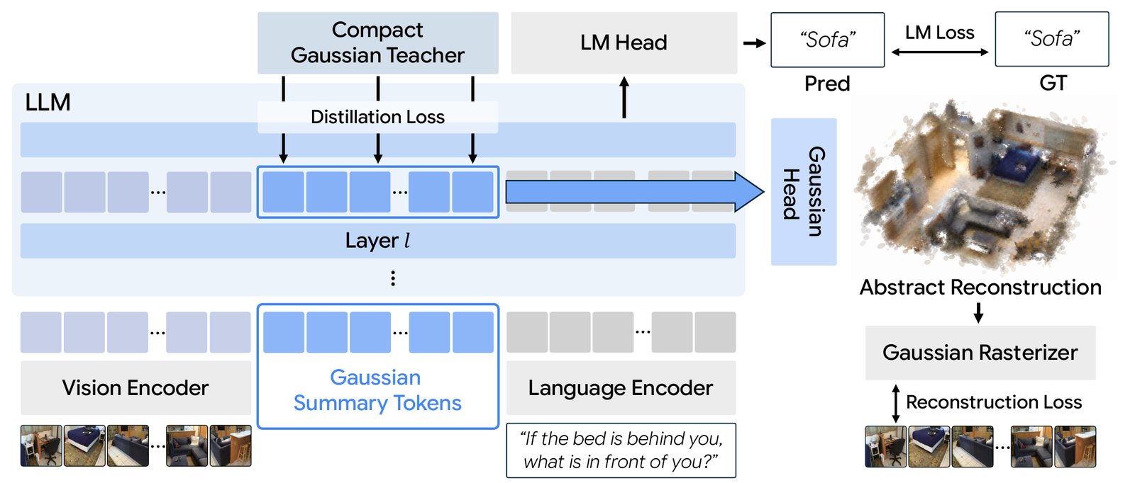
The evidence (reported). The number to trust is the controlled one: same backbone, data and schedule, without the summary tokens.
| Benchmark | Same-data baseline | Imagine3D-LLM |
|---|---|---|
| SQA3D (exact match) | 56.5 | 63.8 |
| ScanQA (exact match) | 26.2 | 29.9 |
| SPAR-Bench (average) | 60.9 | 68.5 |
The ablations isolate the cause well. Feeding the teacher's tokens straight in leaves SQA3D at 56.4; distillation without reconstruction, 56.6; reconstruction alone reaches 63.7, but takes four epochs. The bottleneck matters both ways: 1,296 summary tokens give 61.9, 5,184 give 60.3.
The headlines need that table. On SPAR-Bench it scores 68.5, 5.2 points over 3DThinker-7B and more than 29 over Qwen2.5-VL-72B's 39.4. But training includes a 100K subset of SPAR-7M, the benchmark's own training source, the 72B is zero-shot, and the same-data baseline already scores 60.9. Of the margin over the 72B model, 7.6 points are the method's (reasoned). ScanQA exact match, 29.9, trails Ross3D's 30.8. At inference the decoder is optional but the summary tokens stay: 176.9 ms per SPAR sample against 112.1 ms, and 20.43 GB against 17.09 GB. Code is "Coming Soon". Where WorldCrafter skips explicit reconstruction, Imagine3D-LLM keeps it, but only as a training signal.
What you can run today
| Item | Code | Weights | Licence | Notes |
|---|---|---|---|---|
| Mira-Scene | VAST-AI-Research/Mira-Scene at 18f4265 | Yang-Tian/Mira-Scene | No licence file or declared licence | Mesh stage needs SAM 3D or TRELLIS.2; training data still to come |
| HARMONY | ShufanSun/harmony-release at 36768c5 | Others' models | MIT code; benchmark card says MIT in metadata, CC-BY-NC-4.0 in text | Needs VGGT, SAM 2, Hunyuan3D-2, an image editor, a VLM |
| DAVINCI | None found | None | Preprint CC BY 4.0 | Configuration in the appendix |
| D3GS | None found | None | None | |
| NG-GS | BJTU-KD3D/NG-GS at 7afa887 | None | Inria, non-commercial | Differs from the paper |
| Imagine3D-LLM | "Coming Soon" | None | None | Paper PDF only |
A public repository with no licence file is not open source in any legal sense; I would ask VAST before building on Mira-Scene.
What would change my mind
4 claims above, and what would falsify each
Mira-Scene's 'surpasses GPT-6 Astra' has no metric behind it.
Read from the arXiv paper (v2), which never mentions Astra, and the project page's data file, whose Astra section is six pairs of viewers and one sentence. Any quantitative Astra comparison in a Mira-Scene release falsifies it.
DAVINCI's 4.0× compactness at mean PSNR parity is measured on a mesh it is given, not one it reconstructs.
Inferred from the preprint: the mesh is an input, a real capture has none, and the source of the Ref-NeRF meshes is unstated. If they were reconstructed from the training photos, the asymmetry disappears.
NG-GS's released code does not implement the NeRF-guided method its paper describes.
Read from
scene/ngs_model.pyandtrain.pyat7afa887; I did not run it. A commit that adds ray sampling and the density-weighted mask loss, or a run of this code reproducing 84.7 boundary mIoU on NVOS, falsifies it.Most of Imagine3D-LLM's margin over Qwen2.5-VL-72B on SPAR-Bench comes from training on SPAR data.
Arithmetic on the paper's Tables 3 and 4, resting on its statement that the 60.9 baseline shares the training data. If it did not include the SPAR-7M subset, the claim is wrong.
Sources: the four arXiv papers at the versions linked, HAL hal-05756863v1, the Imagine3D-LLM PDF, and shallow clones at the commits named. Figures are the papers' own, used for commentary.