2026-09-26 · 23 min · slam · state-estimation · robotics · factor-graphs · open-source · explainer
On 23 September 2026 Frank Dellaert posted on X: "After a very busy conference submission
period, I was finally able to build and release GTSAM 4.3!" He pointed at
gtsam.org for the improvements, papers, notebooks and contributor
credits. The 4.3.0 tag itself points at a merge commit dated 18 September. The previous minor release,
4.2, was tagged on 3 September 2023. Three years is a long time for a library that sits
underneath a lot of SLAM, visual odometry and structure-from-motion code, so I cloned it and
counted.
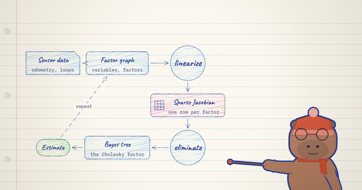
This article does two things. First it explains what GTSAM computes: factor graphs, MAP inference as nonlinear least squares, why sparsity makes that fast, and how elimination and the Bayes tree turn into iSAM2. There is a small pose-graph solver running in the page so you can watch a loop closure pull a drifting trajectory back. Then it goes through 4.3 itself, verified against the tag, the commit log, the release page and the official Python wheel, which I installed and timed.
- license
- custom
- branch
- HEAD
- tests
- 1273 files
- source
- 58.8 MB
- commit date
- 2026-09-18
by size of tracked source at this commit, file counts in brackets; docs, data and vendored trees excluded
local clone, 2026-09-26 at 71a25ca — branch, commit, commitDate, fileCount, hasTests, languages, license, licenseFile, shallow, testFileCount
shallow clone: counts describe the pinned tree, not the history
Why robots think in factor graphs
A robot does not measure its state. It measures relations. The wheel encoders say "I moved about 1 m forward and turned about 30 degrees since the last pose". The camera says "that corner is at this bearing and range from where I am now". The GPS says "you are roughly here". A place-recognition module says "you have been here before". Each of these touches one or two unknowns, never all of them.
A factor graph writes that down literally. It is a bipartite graph with two kinds of node:
- Variables: the unknowns. Robot poses , landmark positions , calibration, IMU biases.
- Factors: one per measurement. A factor is a function of the handful of variables the measurement involves, and it scores how well a guess for those variables explains it.
The graph is a factorisation of the posterior. If each factor is a Gaussian measurement model, the probability of all the unknowns given all the measurements is a product of one term per factor:
Here is the small set of variables factor touches, predicts the measurement from them, is what the sensor reported, and is the squared Mahalanobis norm, the error scaled by the sensor's noise covariance.
This is the same Gaussian bookkeeping as a Kalman filter, with one difference in what is kept. A filter marginalises every past state away as it goes and carries only the latest belief. A smoother keeps the whole trajectory as variables, so a measurement that arrives late, like a loop closure, can correct poses from minutes ago. GTSAM's name says which one it is: Georgia Tech Smoothing and Mapping.
MAP inference is nonlinear least squares
Taking the negative log of that product turns the most probable estimate, the maximum a posteriori (MAP) one, into a sum of squares:
The are nonlinear: they rotate, project and compose poses. So the solver linearises around the current guess, solves a linear least-squares problem for a correction , applies it, and repeats. That is Gauss-Newton; Levenberg-Marquardt adds damping so a bad step can be rejected. Each iteration solves
where each block row of is one factor's whitened Jacobian and its whitened residual. One detail matters for robotics: poses are not vectors. A rotation cannot be updated by adding three numbers to it. GTSAM computes in the tangent space and retracts it back onto the manifold, . The FAST-LIO2 article does the same thing inside an iterated Kalman update; that iteration is also Gauss-Newton on a MAP objective.
The number GTSAM reports as graph.error(values) is half the sum above. It is the number
the widget and every table below print.
Sparsity is the whole trick
has one block column per variable and one block row per factor. Each factor touches one or two variables, so each block row has one or two nonzero blocks. A 10,000-pose graph has a 30,000-column with almost nothing in it. The normal matrix inherits the pattern: block is nonzero only if some factor touches both and . In other words, the sparsity pattern of is the factor graph's adjacency.
The solver never inverts . It factors it, with upper triangular, and back-substitutes. For an odometry chain the factor keeps the chain's shape: is tridiagonal, is bidiagonal, and solving costs time linear in the number of poses.
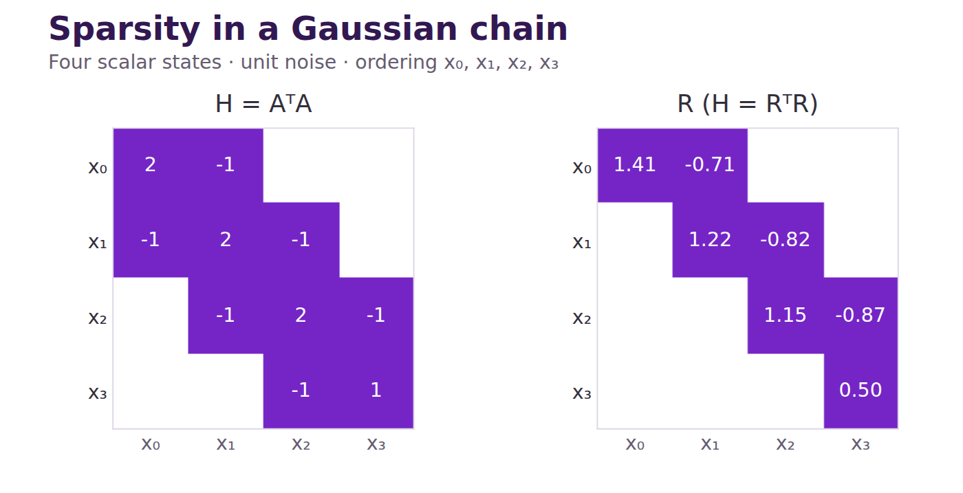
A loop closure breaks the chain. It adds a factor between the first and last pose, so gets two corner blocks, and factoring it in the order creates fill-in: eliminating couples to the last pose, eliminating couples to it, and so on down a whole column of . The order in which variables are eliminated decides how much fill you pay for, which is why GTSAM computes an ordering (COLAMD by default, METIS nested dissection as an option) before it factors anything.
Here is that in a form you can poke. Thirteen poses, twelve 1 m odometry steps with a 30 degree turn each, so the true path is a closed dodecagon. The simulated gyro reads high by a bias you set, plus a little seeded noise:
- position RMSE
- 0.677 m
- gap x12 → x0
- 0.99 m
- σx of x12
- 0.289 m
Squares are factors, shaded by how much error each one carries. With the loop closure off, dead reckoning already satisfies every odometry factor, so the error is zero and there is nothing to optimise; only the ellipses grow. Switch it on and the whole error sits on the one red square. Two or three Gauss-Newton steps later it is shared by all thirteen factors, the loop closes, and σx of x12 collapses. The price shows in the right-hand panel: one extra factor fills a whole column of R.
With the loop closure off, dead reckoning satisfies every odometry factor exactly, so the graph error is zero and there is nothing to optimise; the estimate is simply wrong, and the 1-sigma ellipses grow along the chain. Switch the loop-closure factor on at the default 3 degree bias and the whole error, about 750, sits on that one factor. Gauss-Newton takes it to about 83, then to 11.37 and stops, spreading the residual across all thirteen between factors. The gap between the last pose and the first goes from 0.99 m to zero, position RMSE against the truth drops from 0.677 m to 0.108 m, and the x-sigma of the last pose drops from 0.289 m to 0.049 m. The right-hand panel shows the cost: the one extra factor puts 10 fill-in blocks into .
The solver in the widget is mine and small. Poses are and the correction is
added directly; the between residual is the translation expressed in the first pose's frame
plus the wrapped heading difference. GTSAM's BetweenFactor<Pose2> uses the SE(2)
logarithm and retracts on the manifold. I checked what that costs by feeding the widget's
exact odometry to GTSAM 4.3.0: at the default bias its Levenberg-Marquardt ends at the same
graph error, 11.37, and the same 0.108 m RMSE. Only the starting error differs, 755.55
against the widget's 749.92, because the two residuals disagree far from the optimum.
Elimination, the Bayes tree, and iSAM2
Cholesky on has a graphical reading, and it is the one GTSAM is built on. Eliminating a variable means: take every factor that touches , multiply them together, and split the result into a conditional density on the variables it was connected to (its separator), plus one new factor on alone. Do that for every variable in order and the factor graph becomes a Bayes net, whose conditionals are exactly the rows of . The new factor on is where fill-in comes from.
Group the conditionals into cliques and they form a tree, the Bayes tree, with the last
eliminated variables at the root. That structure is what makes incremental SLAM cheap. A new
measurement touches a few variables; only the cliques on the path from those variables to
the root change. iSAM2 (Kaess et al., IJRR 2012)
detaches that top part of the tree, turns it back into factors, adds the new ones,
re-eliminates just that piece, and re-attaches the untouched subtrees. It also relinearises
lazily: a variable gets a new linearisation point only when its estimate has moved more than
a threshold (0.1 by default in ISAM2Params, checked every 10 updates).
I fed the same thirteen-pose problem to gtsam.ISAM2 one factor at a time and read
getVariablesReeliminated() after each update. Every odometry step re-eliminated 3 or 4 of
the poses. The loop closure re-eliminated all 13. That is the Bayes-tree version of the fill
column in the widget: a loop closure couples the ends, so the whole loop sits under the
root.
Running it: the 4.3.0 wheel
pip install gtsam==4.3.0 pulled a 34 MB manylinux wheel for CPython 3.11 and NumPy 2.4.6.
The script below is the widget's problem in GTSAM itself, with NumPy's generator supplying
the noise, so its numbers differ slightly from the widget's.
# loop.py -- twelve noisy odometry steps around a loop, then one loop closure.
import math
import numpy as np
import gtsam
from gtsam.symbol_shorthand import X

N = 12                                        # 12 steps of 30 deg close the loop
rng = np.random.default_rng(7)
TRUE_STEP = gtsam.Pose2(1.0, 0.0, math.radians(30))
odom_noise = gtsam.noiseModel.Diagonal.Sigmas(np.array([0.05, 0.05, math.radians(2)]))
loop_noise = gtsam.noiseModel.Diagonal.Sigmas(np.array([0.05, 0.05, math.radians(1)]))

graph = gtsam.NonlinearFactorGraph()
graph.add(gtsam.PriorFactorPose2(X(0), gtsam.Pose2(), gtsam.noiseModel.Isotropic.Sigma(3, 1e-3)))
initial, truth = gtsam.Values(), [gtsam.Pose2()]
initial.insert(X(0), gtsam.Pose2())
for k in range(N):
    dx, dy, dth = rng.normal(0, [0.05, 0.05, math.radians(2)])
    odom = gtsam.Pose2(1.0 + dx, dy, math.radians(30 + 3) + dth)   # biased gyro + noise
    graph.add(gtsam.BetweenFactorPose2(X(k), X(k + 1), odom, odom_noise))
    initial.insert(X(k + 1), initial.atPose2(X(k)).compose(odom))    # dead reckoning
    truth.append(truth[-1].compose(TRUE_STEP))

def rmse(values):
    d = [values.atPose2(X(k)).translation() - truth[k].translation() for k in range(N + 1)]
    return math.sqrt(np.mean([v @ v for v in d]))

def solve(g):
    opt = gtsam.LevenbergMarquardtOptimizer(g, initial, gtsam.LevenbergMarquardtParams())
    result = opt.optimize()
    sigma = math.sqrt(gtsam.Marginals(g, result).marginalCovariance(X(N))[0, 0])
    print(f"  graph error {g.error(initial):8.3f} -> {g.error(result):.3f} "
          f"in {opt.iterations()} iterations; RMSE {rmse(result):.3f} m; "
          f"sigma_x(x12) {sigma:.3f} m")

print(f"dead reckoning: RMSE {rmse(initial):.3f} m")
print("odometry only:");  solve(graph)
graph.add(gtsam.BetweenFactorPose2(X(N), X(0), gtsam.Pose2(), loop_noise))  # "I'm back"
print("with loop closure:"); solve(graph)

# The same graph, fed to iSAM2 one factor at a time.
isam, counts = gtsam.ISAM2(), []
for k in range(graph.size()):                 # 0: prior, 1..12: odometry, 13: loop
    g = gtsam.NonlinearFactorGraph(); g.add(graph.at(k))
    v = gtsam.Values()
    if k <= N:
        v.insert(X(k), initial.atPose2(X(k)))
    counts.append(isam.update(g, v).getVariablesReeliminated())
print("iSAM2 poses re-eliminated per update:", counts)
print(f"iSAM2 RMSE after the loop closure: {rmse(isam.calculateEstimate()):.3f} m")
dead reckoning: RMSE 0.405 m
odometry only:
graph error 0.000 -> 0.000 in 1 iterations; RMSE 0.405 m; sigma_x(x12) 0.298 m
with loop closure:
graph error 270.611 -> 4.720 in 3 iterations; RMSE 0.108 m; sigma_x(x12) 0.049 m
iSAM2 poses re-eliminated per update: [1, 3, 3, 4, 4, 4, 4, 4, 4, 4, 4, 4, 4, 13]
iSAM2 RMSE after the loop closure: 0.115 mMeasured, not reported: this is the output of that script on the official wheel. The iSAM2 answer, 0.115 m, is a little worse than batch Levenberg-Marquardt's 0.108 m. That is expected, not a bug: by default iSAM2 takes one Gauss-Newton step per update and relinearises only every 10 updates, trading a few millimetres for bounded work per update.
What is new in 4.3
The release, counted
All of these come from the 4.2 and 4.3.0 tags in a clone of borglab/gtsam. The 4.2.1
and 4.2.2 maintenance releases of 2026 sit on a separate branch and are not ancestors of
4.3.0, so the base is 4.2 itself.
| 4.2 → 4.3.0 | |
|---|---|
| commits | 6,399, of which 1,204 merges and 5,195 not |
| pull requests merged, numbered after 4.2's own #1619 | 755 |
| files changed | 4,582 (+906,555 / −310,325 lines) |
the same, without vendored gtsam/3rdparty and wrap/pybind11 | 2,349 (+753,839 / −52,273) |
C++ and CUDA source (.cpp, .h, .cu) | +190,178 / −33,614 lines |
| Jupyter notebooks in the tree | 4 → 329 (+443,465 lines) |
| distinct author emails / people, after merging aliases and dropping bots | 150 / about 120 |
The notebooks are the largest line count in the release, close to the landing page's count of 328 notebooks in the 4.3 documentation. The work was not evenly spread in time: August 2026 alone has 605 non-merge commits, more than three times any other month that year, and 848 non-merge commits landed between the last pre-release, 4.3a2 on 4 August, and the final tag. That is the "very busy" period.
A C++17 break, and Boost made optional
4.2 compiled as C++11 (cxx_std_11) and required Boost 1.65 or newer. 4.3.0 compiles as
C++17 (cxx_std_17) and makes Boost optional behind two CMake flags,
GTSAM_USE_BOOST_FEATURES and GTSAM_ENABLE_BOOST_SERIALIZATION. Both default to ON in an
ordinary CMake build and OFF inside a ROS 2 colcon build. In gtsam/ outside the vendored
libraries, boost::shared_ptr went from 610 occurrences to 0, boost::optional from 384 to
2, and #include <boost…> lines from 338 to 109.
If you maintain custom C++ factors, this is the part that breaks your build. The project's
own examples/LocalizationExample.cpp shows the migration in one function:
// GTSAM 4.2
typedef boost::shared_ptr<UnaryFactor> shared_ptr;
Vector evaluateError(const Pose2& q, boost::optional<Matrix&> H = boost::none) const override {
  const Rot2& R = q.rotation();
  if (H) (*H) = (gtsam::Matrix(2, 3) << R.c(), -R.s(), 0.0, R.s(), R.c(), 0.0).finished();
  return (Vector(2) << q.x() - mx_, q.y() - my_).finished();
}

// GTSAM 4.3.0
using NoiseModelFactor1<Pose2>::evaluateError;   // keep the Matrix& overloads visible
typedef std::shared_ptr<UnaryFactor> shared_ptr;
Vector evaluateError(const Pose2& q, OptionalMatrixType H) const override {
  const Rot2& R = q.rotation();
  if (H) *H = gtsam::Matrix{{R.c(), -R.s(), 0.0}, {R.s(), R.c(), 0.0}};
  return Vector{{q.x() - mx_, q.y() - my_}};
}
OptionalMatrixType is a plain Matrix* (gtsam/nonlinear/NonlinearFactor.h), so a null
pointer means "no Jacobian requested". The deprecation machinery also moved on by one
version: 4.2's library source mentions GTSAM_ALLOW_DEPRECATED_SINCE_V42 on 43 lines and
4.3.0's on none, while GTSAM_ALLOW_DEPRECATED_SINCE_V43, which defaults to ON, appears on
72. The README's advice is to
turn it off while migrating, to find what will be removed after 4.3. The fixed-lag smoothers
graduated from gtsam_unstable/nonlinear to gtsam/nonlinear; the old headers still exist
and forward to the new ones with a compile-time #warning.
One default changed underneath everyone. GTSAM_SLOW_BUT_CORRECT_BETWEENFACTOR was OFF in
4.2 and is ON in 4.3.0, now described as "Use Local Jacobians in BetweenFactor and PriorFactor
when provided by traits" (PR #2661, merged 11 August). Despite the name, the gtsam.org CUDA
post reports it as a speedup: the exact Jacobian costs a few nanoseconds more per factor but,
on the 10,000-pose w10000 graph, "cut LM time after FAST-Sync by more than half". That is
reported, not measured by me: the flag is compiled in, so the wheel cannot toggle it.
New solvers: multifrontal, CUDA, FAST-Sync, riSAM
MultifrontalSolver. A new linear solver with precomputed elimination structure, packed
storage reused across solves, and TBB-scheduled parallel elimination. It is opt-in:
linearSolverType still defaults to MULTIFRONTAL_CHOLESKY, and the new path is
MULTIFRONTAL_SOLVER.
CUDA, experimental. PR #2706 (merged 20 August) adds gtsam::cuda::SparseLevenbergMarquardtOptimizer,
which takes an ordinary NonlinearFactorGraph, linearises on the CPU and ships the sparse
Jacobian to the GPU for the solve, with cuDSS or preconditioned conjugate gradients.
gtsam::cuda::SfmLevenbergMarquardtOptimizer goes further for bundle adjustment and keeps
the whole Levenberg-Marquardt loop on the GPU, down to a dense Cholesky of the Schur
complement. The release page's chart summarises the benchmarks:
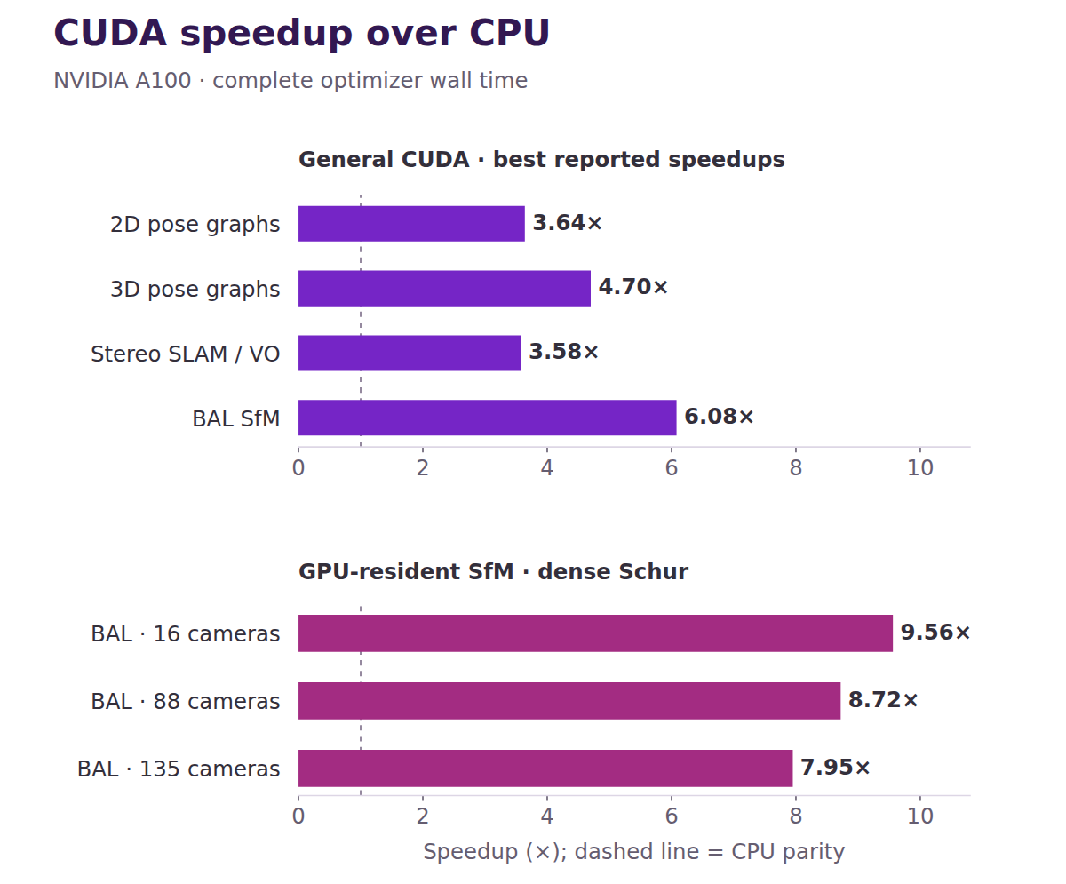
On those BAL problems the best CPU time was 1.069 s, 3.398 s and 4.438 s against 0.112 s,
0.390 s and 0.558 s on the GPU. The same post notes the flip side: tiny problems are
dominated by setup and launch overhead and can be faster on the CPU. None of this is in the
PyPI wheel. The standard 4.3.0 wheels do not include gtsam.cuda (I checked: no cuda
attribute), and using it from Python means building GTSAM and its wrapper yourself with
GTSAM_ENABLE_CUDA=ON.
FAST-Sync (PR #2634, 8 August) is an initialiser, not an optimiser. Local solvers like
Levenberg-Marquardt need a start inside the right basin, and the usual cheap start, chaining
relative measurements along a spanning tree, accumulates error along every path. FAST-Sync
relaxes the group constraint, solves one structured linear least-squares problem over all
the measurements with a nested-dissection ordering, and projects each result back onto the
group. The Python wheel exposes it for seven groups: fastSyncRot2, fastSyncRot3,
fastSyncPose2, fastSyncPose3, fastSyncSimilarity2, fastSyncSimilarity3 and
fastSyncSL4.
riSAM (PR #2409, merged 16 August, by Dan McGann) is a robust variant of iSAM2. The
header describes it as solving "each incremental update using an efficient form of Graduated
Non-Convexity to reject outliers while maintaining robustness to initialization". That is
the problem the widget above does not have: its one loop closure is correct. A real
place-recognition module produces wrong ones, and a single wrong loop closure in plain least
squares drags the whole map. riSAM is C++ only at 4.3.0: no .i wrapper file mentions it,
so it is not in the Python module.
I timed two of them on a 10,000-pose graph
The wheel ships the w10000 pose-graph dataset: 10,000 poses and 64,311 between
factors. I added a prior on the first pose and ran Levenberg-Marquardt from the file's own
initial guess and from fastSyncPose2, each with the default linear solver and the new
multifrontal one. Median of three runs, on a 4-vCPU Intel Xeon at 2.10 GHz:
| start | linear solver | LM iterations | final error | wall time |
|---|---|---|---|---|
| file's initial guess (error 27,603,147.8) | MULTIFRONTAL_CHOLESKY, default | 8 | 144.87 | 1.87 s |
| file's initial guess | MULTIFRONTAL_SOLVER, new | 8 | 144.87 | 2.96 s |
| FAST-Sync, 0.36 s (error 23,455.8) | MULTIFRONTAL_CHOLESKY | 10 | 144.87 | 2.35 s |
| FAST-Sync | MULTIFRONTAL_SOLVER | 10 | 144.87 | 2.93 s |
Two results I did not expect, and neither is the release's fault. FAST-Sync starts three
orders of magnitude closer, 23,455.8 against 27.6 million, but on this graph the file's
guess was already inside the basin, so both starts reach the same 144.87 and FAST-Sync
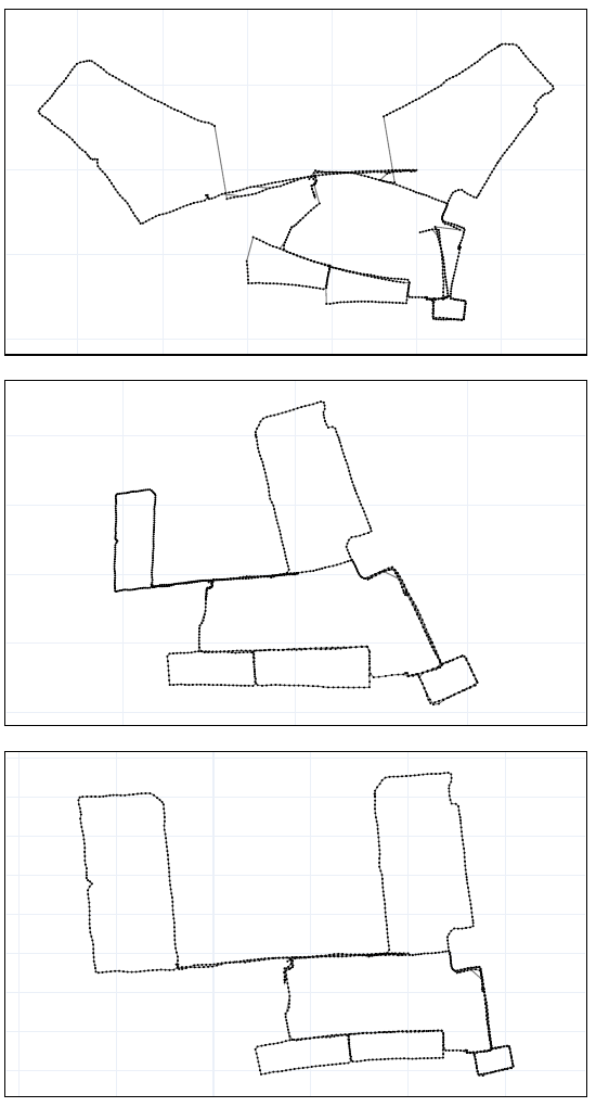
costs two more iterations. Its payoff is on graphs where the cheap start is in the wrong
basin, which the MIT figure shows and this dataset does not. And the new multifrontal
solver was slower here, 2.96 s against 1.87 s. The wheel is built with GTSAM_WITH_TBB
defaulting to OFF (.github/scripts/python_wheels/cibw_before_all.sh), and the library in
it links no TBB, so its parallel elimination is not in play. This says nothing about a C++
build with TBB, which I did not measure.
The estimation modules
Most of the new lines are new capability rather than new solvers. Each of these has a module, Python bindings and notebooks, and most have a paper:
| area | what landed | paper |
|---|---|---|
| navigation | Gal(3) and NavState Lie-group IMU preintegration, invariant and equivariant EKFs, legged-robot estimators | Four Simple Proprioceptive Estimators for Legged Robots |
| GNSS | pseudorange, carrier-phase, Doppler, differential, double-difference and undifferenced factors, with lever-arm variants | Kosuke Inoue's RTK evaluation on gtsam.org |
| continuous time | white-noise-on-acceleration Gaussian-process priors and interpolation, WnoaFactorGraphPose3 and friends | Smoothing Out the Edges |
| constrained | LP, QP and QCQP problems; augmented-Lagrangian, penalty and active-set optimisers | |
| certifiable | SDP relaxations and a Riemannian-staircase optimiser for rotation averaging, pose graphs and landmark SLAM | Certifiable Factor Graph Optimization, chordal sparsity |
| hybrid | discrete-continuous elimination, hybrid Bayes trees and smoothing with pruning | Variable Elimination in Hybrid Factor Graphs |
| robust | riSAM | riSAM |
The certifiable module is the one to watch if you ship pose-graph optimisation. Everything
above it, the widget included, finds a local minimum and cannot tell you whether it is the
global one. A certifiable solver can, when the relaxation and its certificate conditions
hold. New geometry types came with these: Gal3, SL4, ExtendedPose3,
FundamentalMatrix and Cal3f did not exist in 4.2.
Python
The wheel now carries a PEP 561 py.typed marker (PR #2777) and generated .pyi stubs, so
an editor or mypy sees real signatures for the C++ types. It installed alongside NumPy
2.4.6 without complaint. Coverage is broad but not total: FAST-Sync, the GNSS factors, the
Gaussian-process graphs, QP and QCQP, the Riemannian staircase and the hybrid classes are all
importable; riSAM and CUDA are not.
Who did it
Frank Dellaert wrote 1,903 of the 5,195 non-merge commits, under three identities; Varun
Agrawal, who led the hybrid-inference work, wrote 1,473. Together that is about 65%. After
them come leolrg, the account the CUDA pull requests came from and which the site credits
to Ruogu Li (179), Kartik Arcot (127), Rohan Bansal (124), Porter Zach, who expanded the
documentation (101), and Dan McGann of riSAM (81). The release page names research
collaborations with the University of Toronto on the Gaussian processes, David Rosen's group
at Northeastern and Frederike Dümbgen at Carnegie Mellon on certifiable estimation, and
Seoul National University on legged estimation.
There is also a new kind of contributor in the log. 90 of the merged pull requests came from
branches named codex/…; 84 commits name Claude, as author or in a
Co-Authored-By: Claude trailer; and 21 are authored by GitHub's Copilot agent. On 29 July Dellaert added
AGENTS.md, CLAUDE.md and GEMINI.md to the repository root in a commit titled
"Centralize AI agent guidance", and the CUDA blog post ends with a disclosure that AI helped
draft it. None of that changes what the code does, and the log cannot say how much of any
commit an agent wrote; it only records which branches and commits name one.
Where it costs
- Custom C++ factors must be ported. The
boost::optional<Matrix&>signature is gone. It is a mechanical change, but it touches every factor you wrote. - CUDA is experimental and not in the wheel. The speedups are the project's, on an A100, and small problems can be slower on the GPU.
- The wheel has no TBB. If you want the multifrontal solver's parallel elimination,
build from source with
GTSAM_WITH_TBB=ON. - FAST-Sync is not free on a graph that did not need it. On w10000 it saved nothing.
- Everything local is still local. Levenberg-Marquardt and iSAM2 find the nearest minimum; the certifiable module is the tool for knowing whether it is the global one.
The one-paragraph summary
A factor graph writes a robot's measurements as factors on the few unknowns each one touches. MAP inference over it is sparse nonlinear least squares: linearise, solve by factoring rather than inverting, retract on the manifold, repeat. The sparsity pattern is the graph, elimination order decides fill-in, and grouping the eliminated conditionals into a Bayes tree lets iSAM2 redo only the part a new measurement touches, which for a loop closure is the whole loop. GTSAM 4.3 keeps all of that and changes a great deal around it: C++17 with Boost optional, a ported custom-factor API, exact Lie-group Jacobians by default, an opt-in multifrontal solver and CUDA backend, FAST-Sync and riSAM, new navigation, GNSS, continuous-time, constrained, certifiable and hybrid modules, and 329 notebooks, in 6,399 commits from about 120 people and a few agents.