3D reconstruction roundup 2: old geometry, bolted onto feed-forward models

md json mcp

2026-10-06 · 22 min · 3d · slam · gaussian-splatting · point-cloud · vision-language-models · benchmarks · paper · explainer

The first roundup grouped six papers by problem. This week's batch has one shared shape. Each takes a feed-forward geometry model (VGGT, Depth Anything 3, LoGeR, TRELLIS.2, a VLM) and bolts on an idea that predates it: a coarse-to-fine pyramid, a fixed primitive budget, a pose graph, a gravity prior, bundle adjustment, a panorama. For each, the same four questions: what problem, what idea, what evidence, and what you can run.

Item	The old idea	Headline, and what it is measured on	Released
T3lescope	Coarse-to-fine pyramid	Beats GenRecon on all seven ScanNet++ metrics; DA3 keeps the better F@2	Paper; code "coming soon"
PocketSplat	Fixed primitive budget	22.790 dB at 226K Gaussians on DL3DV; 10.20 to 10.95 s on an iPhone	Paper only
CLoSeR	Loop closure, pose graph	VBR mean ATE 36.16 → 11.15 m over LoGeR	Code, no licence file
G3T	Gravity-aligned frames	Camera-to-gravity error under GeoCalib's; ACC −37.9% on 10 TUM RGB-D sequences	Code and weights, no licence
EPO	Bundle adjustment, without tracks	AUC@5 77.1 against 70.9 for VGGT's own BA on ScanNet++	Code, IVC licence
OneCanvas	Panoramic reprojection	SQA3D 65.3, VSI-Bench 71.3, SPBench 72.1	Code and weights, MIT

T3lescope: one generator, applied at every scale

Problem. Generative mesh models such as TRELLIS.2 fill in what the photos barely constrain (glass, gloss, the back of a chair), but they work on one fixed voxel grid. A room or a city block at that grid is mush; tiling it into overlapping cells, as GenRecon does, gives detail but lets distant cells disagree.

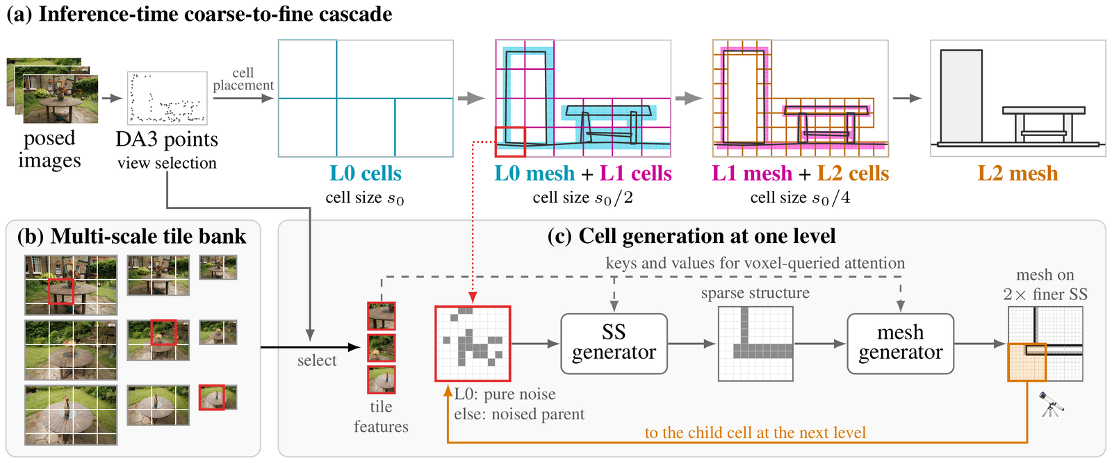
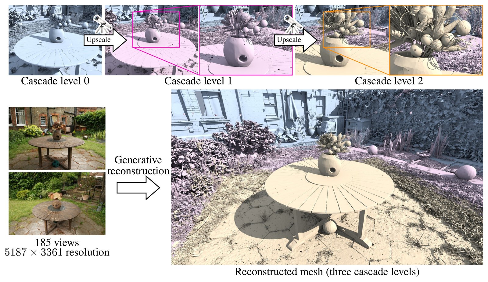
The idea. Run the same generator several times at halving cell sizes, each level starting from the one above. Preferred Networks fine-tune TRELLIS.2 (a sparse-structure flow model, then a mesh flow model, both on a $64^3$ grid per cell) on cells of many physical sizes, never telling it the size. At inference, Depth Anything 3 points place the coarsest cells and pick their views; the depth is used for nothing else. Each finer level takes the parent's decoded surface at twice the resolution, encodes it, noises it to $t_s = 0.8$ and denoises it with finer image features: SDEdit between levels. Images are encoded once, as a pyramid of $512 \times 512$ tiles; each cell reads the level matching its voxel size.

Three-part diagram. Top, an inference-time cascade: posed garden photos give Depth Anything 3 points that place large level-0 cells; the level-0 mesh seeds level-1 cells at half the size, then level-2 cells at a quarter, ending in a detailed mesh of a wall and a table. Bottom left, a multi-scale tile bank: each photo cut into 512-pixel tiles at three pyramid levels. Bottom right, one cell at one level: selected tile features feed a sparse-structure generator and then a mesh generator, starting from pure noise at level 0 and from the noised parent otherwise. — The cascade: Depth Anything 3 points place the coarse cells, each finer level halves the cell size and starts from the noised parent mesh, and every cell reads image tiles at the pyramid level matching its voxel size (T3lescope, Figure 2).

The evidence (reported). On the 25 largest ScanNet++ validation scenes the finest level beats GenRecon on all seven metrics at 32 and 256 views. It does not beat Depth Anything 3 everywhere:

ScanNet++, 32 views	Depth MAE ↓	Normal error ↓	Chamfer (m) ↓	F@2 cm ↑
2DGS (per-scene optimisation)	0.1426	38.376°	0.0723	0.4837
Depth Anything 3	0.0811	28.000°	0.0212	0.7765
GenRecon	0.1175	20.928°	0.0604	0.2846
T3lescope, level 2	0.0565	16.330°	0.0212	0.7155

DA3 keeps the higher F-score at both view counts (0.7882 against 0.7176 at 256 views), and at 256 views also the lower Chamfer (0.0193 against 0.0202) and higher completeness. What T3lescope wins is depth and normals. On Tanks and Temples with 256 views, optimisation still wins F-score clearly (GaussianWrapping 0.650 against 0.354 on the small scenes); the paper says so. The convincing table is city blocks from street photos: Chamfer 0.645 m against 4.858 m for the best baseline. The cascade is load-bearing: starting finer levels from pure noise raises Chamfer from 0.0212 to 0.1051.

Two caveats. "Without per-scene optimisation" is not "fast": a large ScanNet++ scene takes 17 minutes to level 1 and 89 to level 2 on an H200, which the authors call comparable to per-scene optimisation. And glossy and transparent surfaces are shown, not measured: no metric isolates them (reasoned). The project page lists code as coming soon.

Top row: a garden table mesh at cascade levels 0, 1 and 2, each upscale zooming in on the vase of dried flowers, which gains stems and seed heads at each level. Bottom: two of the 185 input photos at 5187 by 3361 pixels and the final mesh, coloured by the level that produced each surface. — Mip-NeRF 360's garden from 185 views: each level re-generates a smaller region in more detail, and the colours mark which level produced each surface (T3lescope, Figure 1).

PocketSplat: an exact Gaussian budget for a phone

Problem. Feed-forward splatting (pixelSplat, MVSplat, DepthSplat) emits one or more Gaussians per input pixel, so the asset's size is set by the input resolution and view count rather than by what the phone can store and render. Their cost volumes also do not fit in an iPhone's memory.

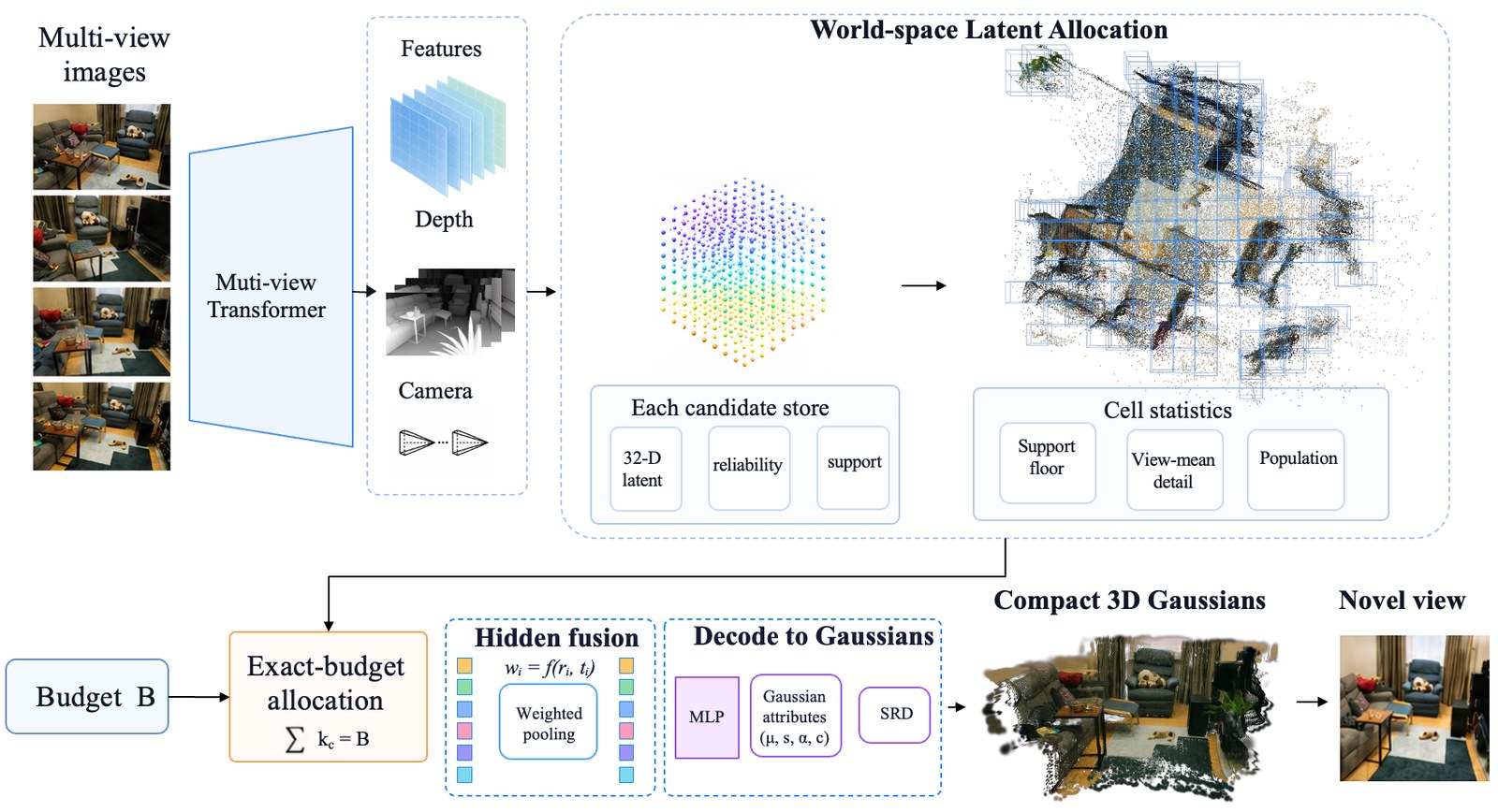
The idea. Predict densely, keep exactly $B$ . A frozen Depth Anything 3 backbone (the iOS export is "six DA3 Core ML stage packages") gives depth and cameras for four views at $252 \times 448$ ; a trained head turns each pixel into a 32-channel latent with a reliability and a support score: 451,584 candidates. Candidates are lifted to world space and binned into cells $2\%$ of the median scene depth wide. Each cell gets a quota from its image detail (the entropy of a $7 \times 7$ patch), divided by the number of views that saw it so repeated evidence is not counted twice, filled by water-filling and rounded so the quotas sum to exactly $B$ . Survivors absorb their cell's pooled latent, and a scale correction widens each Gaussian by about $\sqrt{n_c / k_c}$ , so a cell thinned from $n_c$ to $k_c$ still covers its area.

Pipeline. Four photos of a living room enter a multi-view transformer that outputs features, depth and cameras. Candidates, each storing a 32-dimensional latent, reliability and support, are binned into world-space cells with population, support-floor and view-mean-detail statistics. A budget B drives exact-budget allocation where the cell quotas sum to B, then weighted pooling, an MLP that decodes Gaussian attributes, and spatial responsibility decoding, producing compact 3D Gaussians and a novel view. — Dense candidates are grouped into world-space cells, an allocator splits an exact budget across cells, and only the survivors are decoded into Gaussians, whose scale is then widened for the thinning (PocketSplat, Figure 2).

The evidence (reported). On DL3DV, 226K Gaussians reach 22.790 dB, 1.559 dB over pixelSplat at 1,376,256. Allocation beats a random subset of the same size by 2.19 to 3.69 dB, and the scale correction is worth 3.36 dB at 113K. On the phone (model unnamed), PocketSplat builds an asset in 10.20 to 10.95 s with a 2.64 to 2.89 GB peak; native MVSplat and DepthSplat run out of memory, and a streamed MVSplat takes 42.00 s.

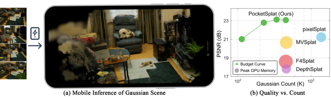
Left, four photos feeding a phone rendering a splatted living room. Right, PSNR against Gaussian count on a log axis: PocketSplat's four budgets climb from about 21 dB at 113K to about 23 dB, above pixelSplat at over a million Gaussians and MVSplat, F4Splat and DepthSplat near 450K, whose bubble sizes show larger peak GPU memory. — The quality-budget curve on DL3DV, bubble area showing peak GPU memory (PocketSplat, Figure 1).

What the budget buys. The post said PocketSplat "decodes only what fits the device budget". The appendix says otherwise: the on-device graph "retains N output rows at all budgets", gives unselected rows an opacity logit of −20, and the PLY writer drops them. The phone does the same work at every budget, hence the flat 10.2 to 11 s. On the GPU a smaller budget is slower (601.8 ms at 113K against 322.3 ms at full), peak memory is 2.705 GB at every budget, and deciding before decoding saves 1.73% of construction time. The budget sets the size of the asset; the memory win comes from not building a cost volume (reasoned). One oddity: the phone's Light row has SSIM 0.6690 and LPIPS 0.2952, identical to the DL3DV 113K row, and Balanced's LPIPS 0.2142 matches DL3DV 226K. Different datasets rarely agree to four decimals twice; with no code, I cannot check (reasoned).

CLoSeR: loop closure for a streaming backbone

Problem. Streaming feed-forward models (LoGeR, CUT3R, TTT3R) keep memory flat over thousands of frames but still drift: nothing tells them they have come back to a place. Submap systems such as VGGT-Long add loop closure, but each VGGT submap has its own scale, so their pose graphs need $\mathrm{Sim}(3)$ , or $\mathrm{SL}(4)$ for VGGT-SLAM, and they align submaps by registering noisy point clouds.

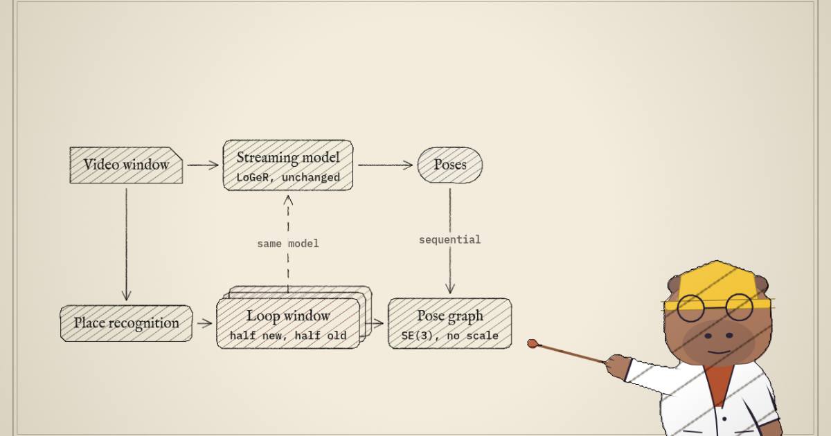
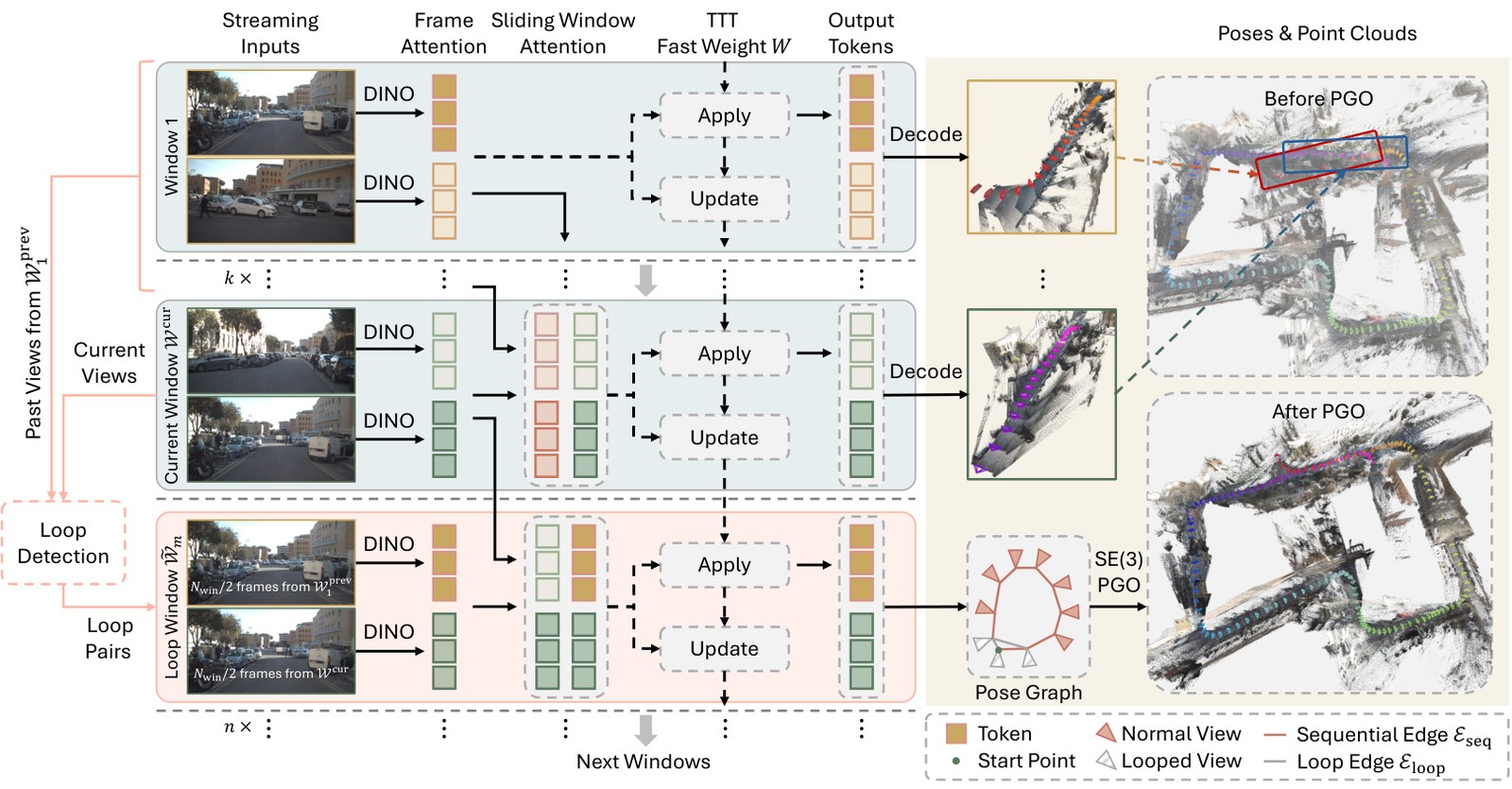
The idea. Use a backbone whose scale is already consistent and ask it for the loop constraint directly. CLoSeR (ETH Zurich) wraps LoGeR without retraining. For each new window it computes SALAD place-recognition descriptors and keeps up to five earlier frames with cosine similarity above 0.7 and at least four windows in the past. It then builds a loop-conditioned window, half current frames and half matched old ones, and runs it through LoGeR, which does not need its inputs to be contiguous. The two halves come back in one frame, so their relative pose is the loop constraint. All poses are then optimised on $\mathrm{SE}(3)$ , with no scale variable:

\min_{\{T_t\}} \sum_{(q,p) \in \mathcal{E}_{\text{seq}}} \left\| \operatorname{Log}\!\left( (T^{\text{seq}}_{qp})^{-1} T_q^{-1} T_p \right) \right\|^2 + \sum_{(j,i) \in \mathcal{E}_{\text{loop}}} \rho_\delta\!\left( \left\| \operatorname{Log}\!\left( (T^{\text{loop}}_{ji})^{-1} T_j^{-1} T_i \right) \right\| \right)

Sequential edges link each frame to its four neighbours; $\rho_\delta$ is a Huber loss that blunts a wrong loop; Levenberg-Marquardt solves it. This is the factor graph GTSAM solves for LiDAR SLAM, with a learned front end in place of scan matching.

System diagram. Streaming windows of street images pass through DINO tokenisation, frame attention, sliding-window attention and test-time-training fast weights to output tokens decoded into poses and point clouds. A loop detection block finds loop pairs from past windows and builds a loop window from half the current window and half a past window, whose poses feed a pose graph. SE(3) pose graph optimisation turns a doubled, misaligned Before PGO point cloud of a city loop into a single consistent After PGO map. — LoGeR streams windows; when SALAD finds a revisit, a loop window of half current and half past frames goes through the same model, and its relative poses become loop edges for an SE(3) pose graph (CLoSeR, Figure 2).

The toy shows what one loop edge does. A 96 m loop of 48 odometry steps with a heading bias you set, dead-reckoned, then solved with one extra edge from the last pose to the first, by Gauss-Newton on $\mathrm{SE}(2)$ :

drift, and one loop edgeSE(2) toy · all numbers computed here

heading bias 1.0°/step

A toy, not CLoSeR: 48 odometry edges with a heading bias, plus one loop edge from the last pose to the first, solved by Gauss-Newton on SE(2) with the first pose held fixed. A heading bias is the error SE(2) can absorb: one loop edge pulls the whole loop back and spreads what is left, so the worst pose ends up far from both ends. Turn on scale drift and the same graph closes the gap but cannot fix the lengths, because it has no scale variable. That is why CLoSeR needs a front end whose scale is already consistent.

In the toy (measured), a bias of 1° per step leaves dead reckoning 12.02 m from its start, with an RMSE of 6.80 m against the truth. One loop edge brings the RMSE to 0.25 m. The worst pose after optimisation, 0.40 m off, is pose 30, far from both ends, because the correction is spread along the loop. Turn on a 25% scale drift and the same graph still closes the gap, but the RMSE stays at 2.98 m with the worst pose 5.31 m off. With no heading bias at all, the optimised loop is worse than dead reckoning (3.04 m against 2.34 m): an $\mathrm{SE}(2)$ graph can only bend the trajectory, not shrink it. That is the bet CLoSeR makes, and the paper measures LoGeR's cross-window scale error on KITTI at 5.8%, against 18.8% for VGGT-Long.

The evidence (reported), ATE RMSE in metres after a $\mathrm{Sim}(3)$ alignment:

Benchmark	LoGeR	CLoSeR	Best other feed-forward
VBR, 7 loops, mean 2.31 km	36.16	11.15	31.12 (LingBot-Map)
KITTI 00–10, mean 2.0 km	25.44	12.79	18.65 (LoGeR*)
Oxford Spires, 14 sequences	6.88	5.26	7.55 (VGGT-SLAM 2.0)
DROID-W, dynamic, 7 sequences	1.44	0.75	0.91 (LingBot-Map)

The ablation supports the scale argument: $\mathrm{Sim}(3)$ instead of $\mathrm{SE}(3)$ gives 13.33 m on VBR, $\mathrm{SL}(4)$ 20.36 m. It costs 7.12 against 7.60 frames a second on an RTX 4090.

What "drift-free" means here. 11.15 m on 2.31 km is less drift, not none. Loop closure only helps where there is a loop: on KITTI's loop-free 01 and 08 CLoSeR scores 41.80 and 26.51 against LoGeR's 41.64 and 26.46. On DROID-W the dynamic-scene SLAM it is named after still wins, 0.23 m. Two small slips: the teaser gives 6.51 m on KITTI 00 where the table has 6.58, and "LoGeR* second best" holds on KITTI but not on VBR. The repository (5230776) has evaluation scripts for all four benchmarks and no licence file.

G3T: predict the pointmap upright

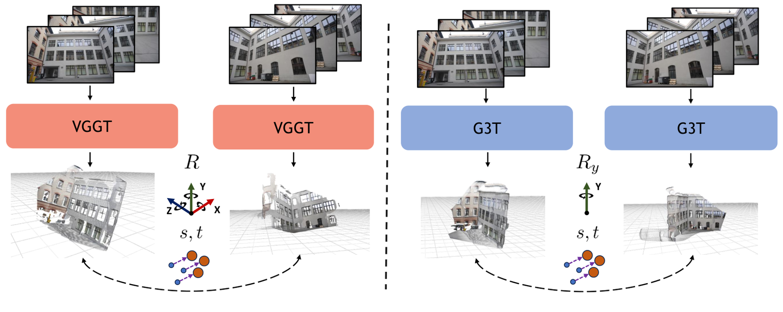
Problem. VGGT predicts every pointmap in the first camera's frame, including its roll and pitch. Two such submaps differ by a full 7-DoF similarity, and any rotation error tilts the floor.

The idea. Predict in a gravity-aligned frame instead. Cornell's G3T fine-tunes all of VGGT so the point head outputs points in the first image's gravity frame (its camera frame with roll and pitch removed, $y$ up). The camera head becomes two: a local head for gravity-to-camera rotation and field of view, and a relative head for yaw (one degree of freedom) and translation. Ground truth comes from five datasets; those not natively upright were aligned with COLMAP's Manhattan-world orientation aligner, so "gravity" in training is partly an estimate. Two upright pointmaps differ by scale, translation and a rotation about $y$ : 5 degrees of freedom. G3T-Long rebuilds VGGT-Long with a Procrustes that solves only that yaw, in the $xz$ -plane, and a pose graph over that 5-parameter group.

Two halves. Left: two VGGT predictions of a courtyard building from different image sets come out tilted relative to a ground grid and are related by a full rotation R plus scale and translation. Right: two G3T predictions of the same building stand upright on the grid and are related only by a rotation about the vertical y axis, plus scale and translation. — Camera-frame pointmaps are related by a 7-DoF similarity; gravity-aligned ones only by scale, translation and yaw, which is what G3T-Long's alignment exploits (G3T, Figure 2).

The evidence (reported). On 7Scenes from one view, the first camera's gravity error falls from 6.78° (GeoCalib) to 1.92° (G3T's local head), and structure accuracy stays at VGGT's level. G3T-Long against VGGT-Long on ten TUM RGB-D sequences:

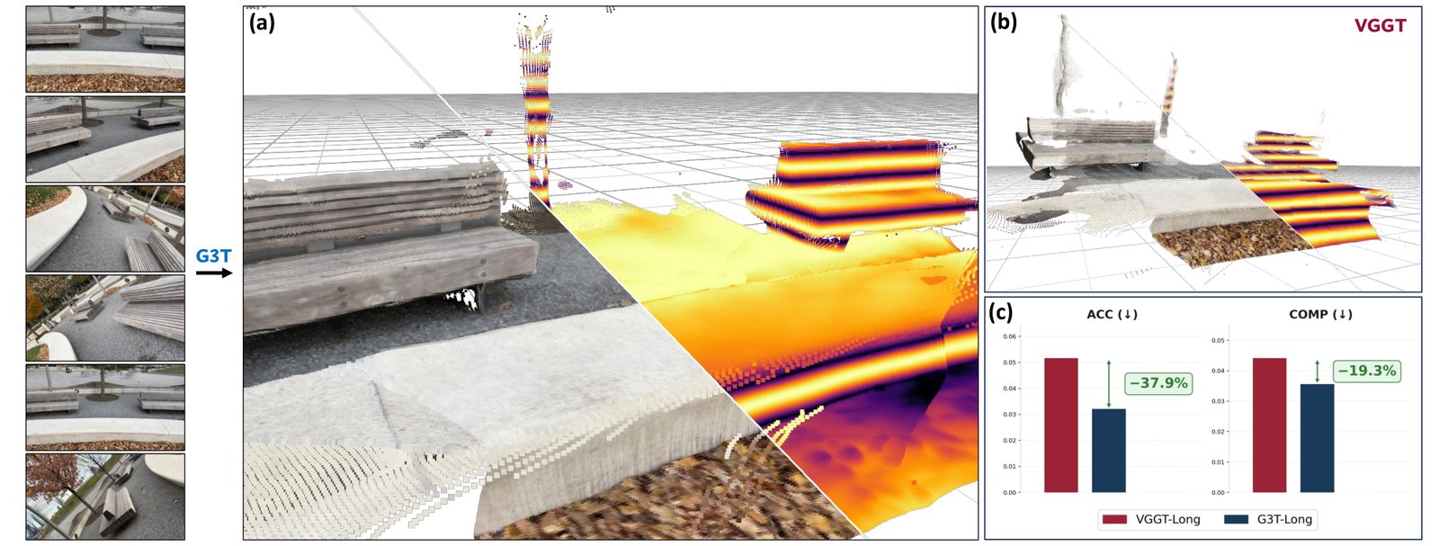
Left, six photos of park benches. Centre, the G3T pointmap of the benches on a level ground grid, half of it coloured by height in flat bands on the ground. Top right, VGGT's pointmap of the same scene, tilted, with height colours sweeping across the ground. Bottom right, bar charts of ACC and COMP for VGGT-Long and G3T-Long, marked minus 37.9 percent and minus 19.3 percent. — Uprightness shown by height colour: flat bands on G3T's ground, a gradient on VGGT's. The bars are medians over ten TUM RGB-D sequences (G3T, Figure 1).

I recomputed the bars from the paper's Table 4 (measured): they are medians over the ten sequences, ACC 0.0515 to 0.032 and COMP 0.044 to 0.0355. The mean ACC improves more, 0.0829 to 0.0386, carried by the long pioneer_slam runs. Rotation error is worse with G3T-Long on two of ten (fr1/360: 19.309° against 16.320°). Two limits: the long-sequence test is indoor TUM RGB-D against VGGT-Long only, with none of the loop-closing systems above, and "regardless of input image orientation" has failures the paper shows, close-ups of floors and a cabinet shot sideways. The paper is from May. Neither the repository nor the Hugging Face weights declare a licence, and VGGT's released 1B checkpoint is CC BY-NC 4.0.

EPO: bundle adjustment on edges instead of tracks

Problem. VGGT's poses are fast and rough. Its own fix, a tracker plus bundle adjustment, needs point tracks, takes minutes, and its refinement variant wants a GPU with at least 40 GB.

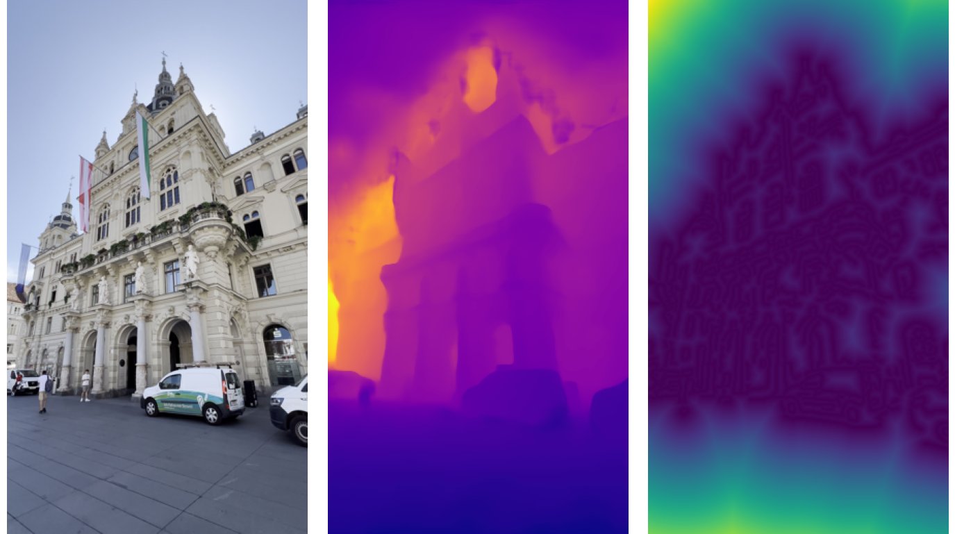
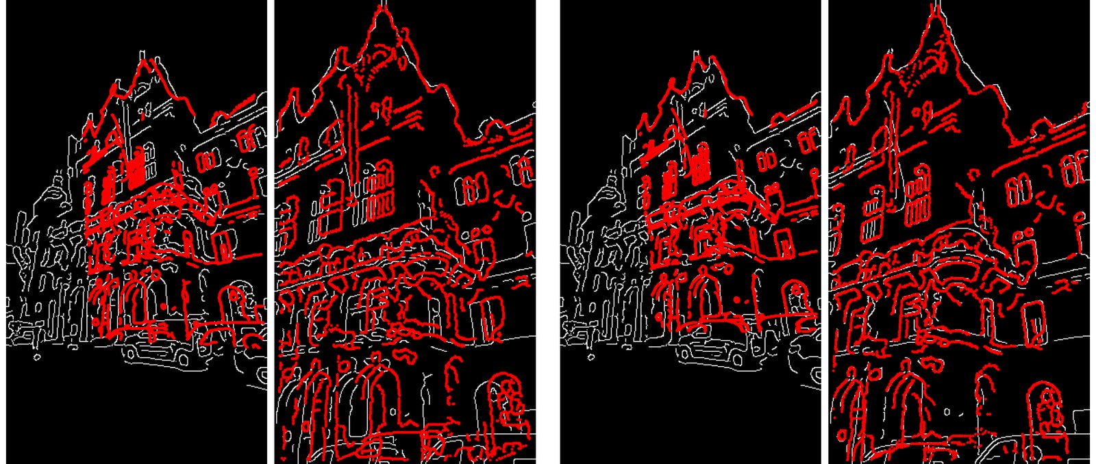
The idea. Align edges instead of matching points. For each image, EPO (Graz) takes a Canny edge map and its distance transform, in which each pixel holds the distance to the nearest edge. Edge pixels of image $i$ are lifted with the model's depth and projected into image $j$ , and the distance transform there says how far each one landed from an edge:

\mathcal{L}_{ij} = \frac{1}{|E_i|} \sum_{p \in E_i} \mathcal{H}\big(\min(\mathrm{DTF}_j[\pi_{i \to j}(p)],\, \lambda)\big) + (i \leftrightarrow j)

with $\mathcal{H}$ a Huber loss, summed over image pairs that reproject consistently. The loss is differentiable everywhere, so AdamW does the work: first poses (through a small MLP, plus a per-camera translation offset) and focal length, then a per-pixel affine correction of depth, stopping when the 95th-percentile pose change goes quiet. No detector, matcher or track.

Three panels of Graz Town Hall: the photo, VGGT's predicted depth map in purple to orange, and the distance transform of the photo's edges, dark along every edge and brightening away from them. — Input image, VGGT's raw depth, and the distance transform field the edge loss samples (EPO, Figure 2).

Four panels of the town hall's white edge map with another view's edges reprojected in red. In the first pair, with VGGT's initial poses, the red edges sit visibly offset from the white ones; in the second pair, after EPO, they lie on top of them. — Edges from one view reprojected into another with VGGT's initial poses and depth (left pair) and after EPO's refinement (right pair) (EPO, Figure 3).

The evidence (reported), AUC at 5°, with total wall-clock time:

	VGGT	+ VGGT's BA	+ track refinement + BA	+ EPO
ScanNet++ (20 scenes)	55.6	70.0, 171.6 s	70.9, 303.5 s	77.1, 52.1 s
TerraSky3D (9 scenes)	56.8	71.1	75.5	79.2
Mip-NeRF 360 (7 scenes)	72.2	85.5	87.8	90.5

It also lifts MapAnything (ScanNet++ 37.3 to 60.4) and $\pi^3$ (70.0 to 80.3). Four caveats. The baselines are VGGT's own tracker-based BA, not COLMAP or GLOMAP. The refinement baseline was timed on an H200 and EPO on an RTX 4090. The reprojection-error table compares EPO's edge-to-edge distance with BA's point-to-keypoint error, two different quantities. And EPO loses outright on one scene, Munich Marienplatz (68.1 against 78.6). Splats trained from EPO's poses reach 23.93 dB on Mip-NeRF 360, against 26.69 from COLMAP poses. The repository has since moved past the paper: v1.4, on VGGT-Omega with radial distortion, reports a mean AUC@5 of 85.7 across four datasets, README numbers not in the paper. The licence is IVC's own: commercial use is allowed "after information to IVC".

OneCanvas: the whole room as one panorama

Problem. A VLM asked about a room sees 32 frames as 32 separate images. Most 3D VLMs add a geometry encoder or scale up spatial QA data.

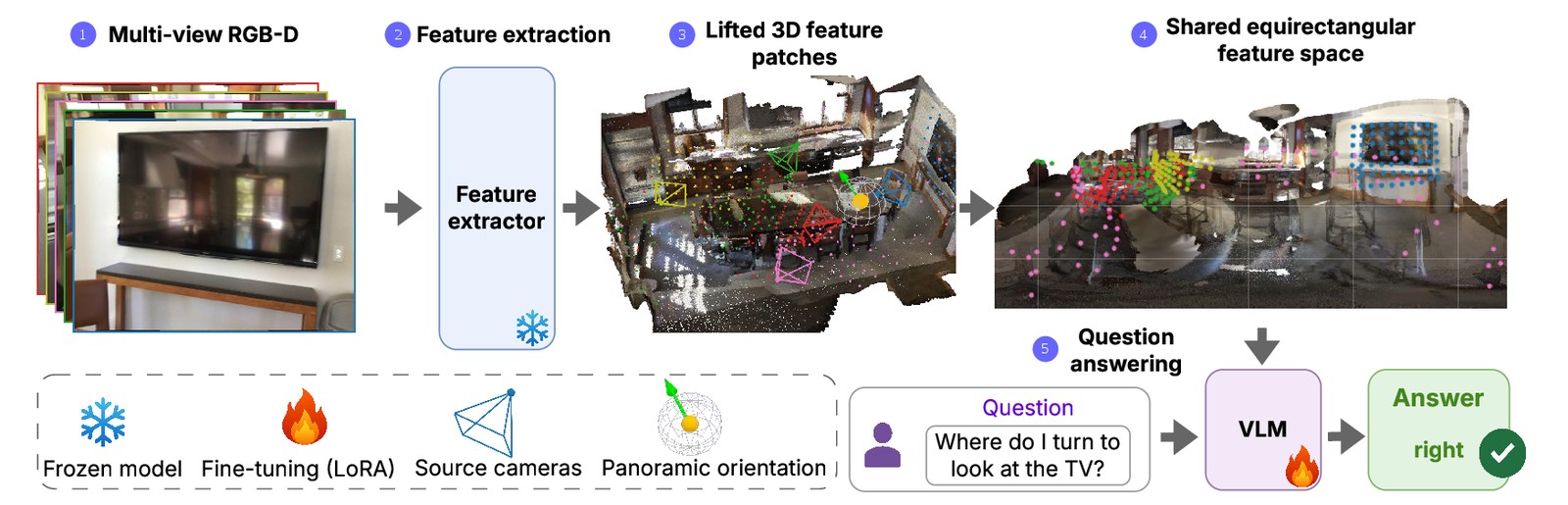
The idea. Put every patch where it is. Qwen3-VL's frozen vision encoder embeds each frame; each patch token is lifted to 3D with its depth and pose, then placed at its continuous longitude and latitude as seen from a chosen origin, the agent's pose for situated questions. Those two angles go into the model's existing rotary position axes for width and height, and the frame index into the temporal axis. Overlapping patches stay separate tokens. A 136-channel sinusoidal code of each patch's metric offset, through a small MLP, puts back the depth the angles lost. Training is two LoRA stages: synthetic spatial tasks built by placing real patches on an empty canvas (rank 256), then QA (rank 64).

Pipeline in five steps: multi-view RGB-D frames of a living room; a frozen feature extractor; feature patches lifted into a 3D point cloud with source cameras and a panoramic origin; a shared equirectangular feature space; and question answering, where the question 'Where do I turn to look at the TV?' goes to a VLM marked as LoRA fine-tuned, which answers 'right'. A legend marks frozen models with a snowflake and LoRA fine-tuning with a flame. — Patches are lifted with depth and pose and placed on one equirectangular canvas around a chosen origin; the vision encoder is frozen, the language model is LoRA fine-tuned (OneCanvas repository README).

The evidence (reported): SQA3D 65.3 exact match, 2.3 over Ross3D; VSI-Bench 71.3, with route planning 12.3 points clear at 60.8; SPBench 72.1 zero-shot, 4.8 over SpaceMind; "an order of magnitude less training compute".

Three corrections to the post. The VLM is not frozen; only the vision encoder is, and its own figure marks the language model as fine-tuned. The canvas reads ground-truth sensor depth and poses; with Depth Anything 3 estimates instead the scores are 64.9, 70.0 and 71.3. And the panorama alone does not carry the result. In the VSI-Bench ablation, at matched LoRA capacity, the base VLM on raw frames scores 65.5 and "panorama only" 65.3; the 3D position code takes it to 68.5 and the curriculum to 71.3. The gain is the metric embedding and the synthetic pretraining, laid out on a panorama (reasoned).

SPBench's headline is the mean of its single-image and multi-view averages (81.5 and 62.8 give 72.1). Every baseline's overall fits that rule except SpaceMind's: its 73.8 and 59.7 average 66.75, not the 67.3 listed (measured). VSI-Bench is not zero-shot: stage 2 trains on VSI-Bench-style data. The released checkpoint scores 65.53, 71.16 and 74.41 by the README's protocols, and SQA3D drops from 65.3 to 61.2 if the canvas sits at the scene centre instead of the agent. Code and weights are MIT.

Briefly

Lyra 2.0 (NVIDIA) turns one image into a walkable world: a long camera-controlled video, with per-frame geometry used only to retrieve past frames, trained on its own degraded outputs so drift gets corrected, then lifted to 3D by a fine-tuned feed-forward model. It is not new: weights came out in April, the GUI and training code in July. "100% open source" holds for the Apache-2.0 code. The weights are under NVIDIA's Internal Scientific Research and Development Model License, which forbids production use and redistribution. WorldCrafter benchmarks against it.

EditHero is a benchmark of 457 part-level edit chains (2,755 edits, 252 objects, up to 30 turns) with an exact target after every turn, assembled from a part library. Its finding: whole-object metrics reward doing nothing (a no-op beats every learned editor on whole-object F-score, LPIPS and PSNR); learned editors follow 0.13 to 0.36 of instructions on the 55-chain comparison set; code-writing LLM agents keep the rest of the mesh intact and reach 0.62 (Opus 5.5), but take 1.5 to 6 minutes an edit against 20 to 50 s. The engine and data are promised, not released.

Texture Space Material Diffusion (NVIDIA) fine-tunes Wan 2.1-1.3B to denoise PBR maps (base colour, height, roughness, metalness) directly in a mesh's UV space, so there are no views to disagree. Photos are projected into texture space as partial observations; 8K comes from generating at 2K and refining shifted crops. It needs a mesh with non-overlapping UVs and camera poses. The source link on the project page is commented out, and git clone of NVlabs/texdiffusion returns "Repository not found" (measured).

image-blaster reconstructs nothing. It is MIT-licensed Claude Code skills and scripts that chain hosted models. Claude reads the photo and lists the movable objects; an image editor (Nano Banana or GPT Image 2) erases them to a clean plate; World Labs' Marble 1.1 turns the plate into a Gaussian splat world with a collision mesh; each object is re-imaged and meshed by Hunyuan 3D on FAL (50,000 faces by default); ElevenLabs effects on FAL add sound; a React viewer plays it. Every 3D asset is generated, from one view, by a paid API.

What you can run today

Item	Code	Weights	Licence
T3lescope	"Coming soon"	None	Paper CC BY 4.0
PocketSplat	None found	None	arXiv licence only
CLoSeR	`MoyangLi00/CLoSeR` at `5230776`	LoGeR's and SALAD's	No licence file
G3T	`g3t-paper/g3t` at `193ce19`	`thatbrguy/g3t`	None declared; fine-tune of VGGT
EPO	`mattiadurso/EPO` at `13bee33`	Uses VGGT and others	IVC, commercial use after informing IVC
OneCanvas	`baranowskibrt/onecanvas` at `5c9c587`	`BaranowskiBrt/OneCanvas-Qwen3-VL-8B`	MIT

A repository with no licence file is not open source in any legal sense; ask before building on CLoSeR or G3T. For where a feed-forward model's metres come from on a robot, see Depth Anything 3 in ROS 2.

What would change my mind

2 claims above, and what would falsify each

PocketSplat's output budget does not reduce on-device compute.
Read from the paper's Appendix D (all N rows kept, unselected opacity −20) and Tables 2 and 6, which show flat phone times and a 2.705 GB peak at every budget. A deployment that skips unselected rows and runs faster at smaller budgets falsifies it.
OneCanvas's panorama alone adds nothing on VSI-Bench; the 3D position code and curriculum do.
Read from the paper's Table 4: base VLM 65.5, panorama only 65.3. If those rows were not trained at matched settings, as the caption says they were, the comparison does not hold.

Sources: the six arXiv papers at the versions linked, the EditHero paper (arXiv 2610.02298), the Texture Space Material Diffusion project page and arXiv 2609.37654, and shallow clones of the repositories at the commits named. Figures are the papers' and READMEs' own, used for commentary.