FAST-LIO2 from scratch: LiDAR-inertial odometry you can actually reproduce

2026-06-28 · 36 min · slam · lidar · state-estimation · point-cloud · explainer

FAST-LIO2 is the LiDAR-inertial odometry I keep coming back to: it's accurate, it runs at 100 Hz on a laptop, it survives 1000 deg/s rotations, and the whole thing is one tight loop around a Kalman filter. But the official code is a maze of templates, and the cleanest annotated fork is in Chinese. So this is the article I wanted: what FAST-LIO2 actually does, derived from first principles, with real code — and a path to rebuild the core without ROS, because once you can do that, you understand SLAM.

If the Kalman filter isn't fresh, read my Kalman piece first — FAST-LIO2 is exactly the "iterated, error-state, on-manifold" filter that article ends on, fed by a high-rate IMU and corrected by thousands of LiDAR points per scan.

The whole system in one loop

The problem: a LiDAR gives you ~100k 3D points per scan at 10 Hz, but a scan takes ~100 ms during which the sensor moves, so the points are distorted; and LiDAR alone is slow to register and fragile under fast motion. An IMU gives you 200–1000 Hz acceleration and angular velocity — great for short-term motion, but it drifts. Fuse them tightly and each fixes the other's weakness.

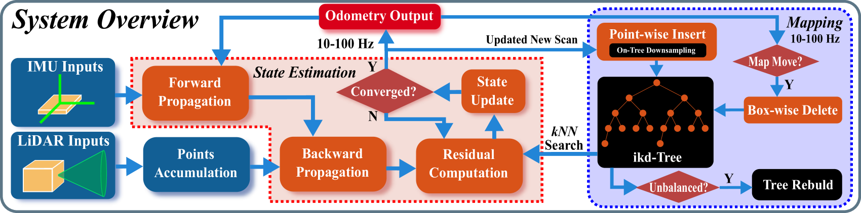
FAST-LIO2 system overview: IMU and LiDAR inputs feed forward propagation, points accumulation, backward propagation, residual computation, and an iterated state update that loops until converged; on the right an ikd-Tree map handles point-wise insert, box-wise delete, and kNN search. — FAST-LIO2's system overview (paper, Figure 1). Left: the state-estimation loop — IMU forward propagation, point accumulation, backward-propagation deskew, point-to-plane residual, iterated state update, repeat until converged. Right: the ikd-Tree map — incremental insert with on-tree downsampling, box-wise delete as the map window moves, and kNN search feeding the residual.

Before the math, here's the cycle as a sequence — what each stage does and, just as important, why it has to be there. It runs once per LiDAR scan; the IMU drives the prediction in between:

FAST-LIO2 cycle · one scan @ LiDAR rate

1. IMU in

What: Read the next batch of 200–1000 Hz accelerometer + gyro samples.

Why: The IMU is the only thing fast enough to describe motion within a 100 ms LiDAR sweep.

Two contributions set FAST-LIO2 apart from its predecessor:

Direct registration. No edge/plane feature extraction — it registers raw points to the map by point-to-plane residuals. Less to tune, and it uses all the geometry.
The ikd-Tree. An incremental k-d tree that inserts, deletes, downsamples, and re-balances in place, so the map updates in real time instead of being rebuilt.

Underneath both is a tightly-coupled iterated error-state Kalman filter on a manifold. Let's build it piece by piece. I'll quote C++ from zlwang7/S-FAST_LIO — a clean reimplementation that writes the filter out explicitly instead of hiding it in template magic — and give simplified NumPy alongside.

The state lives on a manifold

You can't store an orientation as a 3-vector and add to it — rotations live on the manifold $SO(3)$ . FAST-LIO2 tracks a 24-dimensional nominal state but a 23-dimensional error state (and covariance), because each $SO(3)$ rotation needs 3 tangent dimensions, not the 4 of a quaternion, and gravity lives on the sphere $S^2$ (2 dimensions). The state is:

\mathbf{x} = \big[\ \mathbf{p},\ \mathbf{R},\ \mathbf{R}_{L}^{I},\ \mathbf{t}_{L}^{I},\ \mathbf{v},\ \mathbf{b}_g,\ \mathbf{b}_a,\ \mathbf{g}\ \big]

position, attitude, LiDAR→IMU extrinsic rotation and translation, velocity, gyro bias, accel bias, and gravity. In the clean code that's one manifold declaration:

// include/use-ikfom.hpp  — 24-D nominal, 23-D tangent
MTK_BUILD_MANIFOLD(state_ikfom,
  ((vect3, pos))      ((SO3, rot))
  ((SO3, offset_R_L_I)) ((vect3, offset_T_L_I))
  ((vect3, vel))      ((vect3, bg)) ((vect3, ba))
  ((S2, grav)));

We update on the manifold with $\boxplus$ (retraction) and measure differences with $\boxminus$ — for the $SO(3)$ part, $\mathbf{R}\boxplus\delta = \mathbf{R}\,\mathrm{Exp}(\delta)$ and $\mathbf{R}_1\boxminus\mathbf{R}_2 = \mathrm{Log}(\mathbf{R}_2^{\!\top}\mathbf{R}_1)$ . Everything else is ordinary vector $+/-$ .

Forward propagation: ride the IMU

Between LiDAR scans, the IMU drives the state forward. The continuous kinematics are the standard strapdown model — position integrates velocity, attitude integrates de-biased angular velocity, velocity integrates de-biased, gravity-corrected acceleration:

\dot{\mathbf{p}} = \mathbf{v}, \qquad \dot{\mathbf{R}} = \mathbf{R}\,(\boldsymbol{\omega}_m - \mathbf{b}_g)^\wedge, \qquad \dot{\mathbf{v}} = \mathbf{R}(\mathbf{a}_m - \mathbf{b}_a) + \mathbf{g},

with the biases doing a slow random walk. That's get_f verbatim:

// f(x,u): continuous-time kinematics
vect3 omega      = in.gyro - s.bg;            // ω = ω_m − b_g
vect3 a_inertial = s.rot * (in.acc - s.ba);   // R(a_m − b_a)
res(i)      = s.vel[i];                        // ṗ = v
res(i + 3)  = omega[i];                        // Ṙ ← ω
res(i + 12) = a_inertial[i] + s.grav[i];       // v̇ = R(a_m−b_a) + g

The predict step pushes the mean forward by $\mathbf{x} \boxplus (\Delta t\,\mathbf{f})$ and the covariance forward with the error-state Jacobians $\mathbf{F_x},\mathbf{F_w}$ :

\hat{\mathbf{x}} = \mathbf{x}\boxplus(\Delta t\,\mathbf{f}), \qquad \hat{\mathbf{P}} = \mathbf{F_x}\,\mathbf{P}\,\mathbf{F_x}^{\!\top} + (\Delta t\,\mathbf{F_w})\,\mathbf{Q}\,(\Delta t\,\mathbf{F_w})^{\!\top}.

void predict(double &dt, Matrix<double,12,12> &Q, const input_ikfom &i_in) {
    Matrix<double,24,1>  f_     = get_f(x_, i_in);    // 24×1
    Matrix<double,24,23> df_dx_ = df_dx(x_, i_in);    // ∂f/∂x
    Matrix<double,24,12> df_dw_ = df_dw(x_, i_in);    // ∂f/∂w
    x_ = x_.plus(f_, dt);                              // x ⊞ (dt·f)
    // F_x = I + dt·A·df_dx ,  F_w = dt·df_dw  (assembled via the boxplus Jacobian)
    P_ = F_x1 * P_ * F_x1.transpose() + (dt*F_w1) * Q * (dt*F_w1).transpose();
}

In NumPy the shape of it is just:

def predict(x, P, imu, dt, Q):
    f      = get_f(x, imu)              # kinematics above
    F_x, F_w = jacobians(x, imu, dt)   # error-state transition + noise maps
    x = boxplus(x, f * dt)             # advance the mean on the manifold
    P = F_x @ P @ F_x.T + F_w @ Q @ F_w.T
    return x, P

This runs once per IMU sample, and the per-sample poses are cached — we need them next.

Backward propagation: deskew the scan

Because the scan sweeps over time while the platform moves, every point was measured from a slightly different pose. Stack them naively and a flat wall comes out sheared:

scan deskew · motion compensation

platform speed during scan22

Every point lands in the same frame even though the sensor moved between measurements, so a flat wall comes out sheared by the platform's motion. Register this against the map and you'd fight your own motion. Faster motion, worse skew — turn the speed up.

FAST-LIO2 fixes this with backward propagation: walk the cached IMU poses from the scan-end time backward, and transform each point from the pose it was actually sampled at into the scan-end frame. For a point sampled at time $\rho_j$ with the IMU pose $(\mathbf{R}_j,\mathbf{t}_j)$ relative to the scan-end pose $(\mathbf{R}_e,\mathbf{t}_e)$ :

\mathbf{p}^{\text{end}}_j = \mathbf{R}_{L}^{I\,\top}\!\Big(\mathbf{R}_e^{\!\top}\big(\mathbf{R}_j(\mathbf{R}_{L}^{I}\mathbf{p}_j + \mathbf{t}_{L}^{I}) + (\mathbf{t}_j - \mathbf{t}_e)\big) - \mathbf{t}_{L}^{I}\Big)

which is exactly the compensation in UndistortPcl:

M3D R_i(R_imu * Exp(angvel_avr, dt));        // attitude at this point's sample time
V3D T_ei(pos_imu + vel_imu*dt + 0.5*acc_imu*dt*dt - imu_state.pos);
V3D P_compensate = imu_state.offset_R_L_I.conjugate() *
    (imu_state.rot.conjugate() * (R_i * (imu_state.offset_R_L_I * P_i
     + imu_state.offset_T_L_I) + T_ei) - imu_state.offset_T_L_I);

Now every point lives in one consistent frame and it's safe to register against the map.

The measurement: point-to-plane

FAST-LIO2 doesn't extract features. For each deskewed point it transforms it into the world with the current state, finds its 5 nearest map points via the ikd-Tree, fits a plane to them, and the residual is the point-to-plane distance — zero when the point sits exactly on the surface:

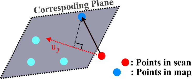
The point-to-plane measurement model: a scan point (red) and the corresponding plane fit from nearby map points (blue), with the plane normal u_j; the residual is the signed distance from the point to the plane. — The measurement model (paper, Figure 2): a scan point (red) is matched to the local plane fit from its nearest map points (blue). The residual is the signed point-to-plane distance along the normal uⱼ — minimized when the estimated pose lands the point on the surface.

For a point $\mathbf{p}$ in the body frame, transformed to world $\mathbf{p}^W = \mathbf{R}(\mathbf{R}_L^I\mathbf{p}+\mathbf{t}_L^I)+\mathbf{p}$ , a plane with unit normal $\mathbf{u}$ and offset $d$ gives residual $z = \mathbf{u}^{\!\top}\mathbf{p}^W + d$ . That's h_share_model:

V3D p_global(s.rot * (s.offset_R_L_I * p_body + s.offset_T_L_I) + s.pos);  // to world
ikdtree.Nearest_Search(point_world, NUM_MATCH_POINTS, points_near, sqDis); // 5 nearest
if (esti_plane(pabcd, points_near, 0.1f)) {                                 // fit plane (a,b,c,d)
    float pd2 = pabcd(0)*x + pabcd(1)*y + pabcd(2)*z + pabcd(3);            // point-to-plane dist
    ...
}
// Jacobian row (w.r.t. attitude θ and extrinsic), residual = −distance
V3D C(s.rot.conjugate() * norm_vec);          // Rᵀu
V3D A(point_I_crossmat * C);                  // (R_L^I p + t_L^I)^∧ Rᵀu
ekfom_data.h_x.block<1,12>(i,0) << norm_p.x, norm_p.y, norm_p.z, A, ...;   // [ u | A | … ]
ekfom_data.h(i) = -norm_p.intensity;          // the residual

The crucial detail: the Jacobian $\mathbf{H}$ is $m\times 12$ — $m$ thousands of points, but only 12 columns (6 for pose, 6 for the extrinsic), because a single LiDAR scan can't observe velocity, biases, or gravity directly. Hold that thought; it's why the next step is fast. In NumPy:

def build_H_z(points_body, x, ikdtree, map_pts, R_LI, t_LI):
    H, z = [], []
    for p in points_body:
        pw = x.R @ (R_LI @ p + t_LI) + x.p          # body → world
        nn = ikdtree.nearest(pw, k=5)               # 5 nearest map points
        n, d = fit_plane(map_pts[nn])               # unit normal, offset
        r = n @ pw + d                              # point-to-plane distance
        if abs(r) < 0.1:                            # keep confident matches
            pI = R_LI @ p + t_LI
            A  = skew(pI) @ (x.R.T @ n)             # ∂r/∂θ  (attitude block)
            H.append(np.concatenate([n, A]))        # [ normal | attitude ]
            z.append(-r)
    return np.array(H), np.array(z)                 # H: m×6 (here), z: m

The iterated update, and the gain that makes it cheap

A single EKF update would linearize the very-nonlinear point-to-plane fit once, at a possibly-wrong pose, and be off. So FAST-LIO2 iterates: re-associate, rebuild $\mathbf{H}$ at the latest estimate, take one Kalman step, repeat until the correction is tiny. Watch the scan snap onto the map:

iterated EKF · point-to-plane registration

iteration

0/5

mean residual

8.0

point-to-plane residual

Each iteration re-associates points to planes at the latest estimate, builds the measurement Jacobian H, and takes one Kalman step dx = K·h + (I−KH)(x⊟x̂). Relinearizing is what makes the very nonlinear point-to-plane fit converge.

Each iteration is

\delta\mathbf{x} = \mathbf{K}\,\mathbf{z} + (\mathbf{I}-\mathbf{K}\mathbf{H})(\mathbf{x}^\kappa \boxminus \hat{\mathbf{x}}), \qquad \mathbf{x}^{\kappa+1} = \mathbf{x}^\kappa \boxplus \delta\mathbf{x},

iterating $\kappa$ until every component of $\delta\mathbf{x}$ drops below $10^{-3}$ . The piece that makes FAST-LIO fast is the reformulated Kalman gain. The textbook form,

\mathbf{K} = \hat{\mathbf{P}}\mathbf{H}^{\!\top}(\mathbf{H}\hat{\mathbf{P}}\mathbf{H}^{\!\top}+\mathbf{R})^{-1},

inverts an $m\times m$ matrix — and $m$ is thousands of points. FAST-LIO uses the information-form identity to rewrite it as

\mathbf{K} = (\mathbf{H}^{\!\top}\mathbf{R}^{-1}\mathbf{H} + \hat{\mathbf{P}}^{-1})^{-1}\mathbf{H}^{\!\top}\mathbf{R}^{-1},

which inverts a $23\times 23$ matrix — the state dimension — no matter how many points there are. That's the whole trick, and in clean code it's one block:

// R is a scalar (LASER_POINT_COV = 0.001), so R⁻¹ = 1/R
auto K_front = (HTH / R + P_.inverse()).inverse();      // (HᵀR⁻¹H + P⁻¹)⁻¹  — 23×23
K = K_front.block<23,12>(0,0) * H.transpose() / R;      // … Hᵀ R⁻¹
Matrix<double,23,1> dx_ = K * dyn_share.h               // K z
       + (Matrix<double,23,23>::Identity() - K*H) * dx_new;  // (I−KH)(x ⊟ x̂)
x_ = x_.boxplus(dx_);
// convergence: every |dx_[j]| < epsi (0.001); then update covariance
P_ = (Matrix<double,23,23>::Identity() - K*H) * P_;

The same loop in NumPy, with the cheap gain spelled out:

def update_iterated(x, P, points_body, ikdtree, map_pts, R=1e-3, max_iter=4, eps=1e-3):
    x_prior = x.copy()
    n = P.shape[0]                                   # 23 (error-state dim)
    for _ in range(max_iter):
        H, z = build_H_z(points_body, x, ikdtree, map_pts, R_LI, t_LI)  # relinearize
        # information-form gain: invert (state × state), independent of len(z)
        S = H.T @ H / R + np.linalg.inv(P)           # n×n
        K = np.linalg.solve(S, H.T) / R              # K = S⁻¹ Hᵀ R⁻¹
        dx = K @ z + (np.eye(n) - K @ H) @ (-boxminus(x, x_prior))
        x  = boxplus(x, dx)
        if np.max(np.abs(dx)) < eps:
            break
    P = (np.eye(n) - K @ H) @ P
    return x, P

That's the engine. The converged $\mathbf{x}$ is your odometry output, published at LiDAR rate.

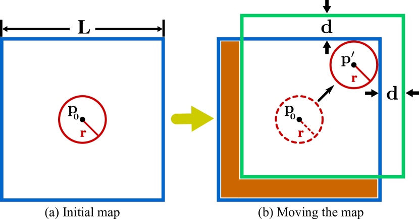
The map: an incremental k-d tree

The nearest-neighbor search in the measurement step is the hot path, and the map is growing and moving. A static k-d tree would be rebuilt every scan — fatal. The ikd-Tree instead inserts points in place, downsamples on the tree, deletes whole regions with one box-wise delete as the local map window slides with the sensor, and lazily re-balances only the subtrees that get lopsided:

ikd-Tree · incremental map with a moving window

active map points

window

bounded

query

kNN, balanced

A static k-d tree would have to be rebuilt from scratch every time the map changed. The ikd-Tree instead inserts and deletes points in place, does voxel downsampling on the tree itself, removes whole regions with one box-wise delete as the window slides, and lazily re-balances only the subtrees that get lopsided — so a moving robot keeps a bounded, balanced map and the nearest-neighbor search in the measurement step stays cheap.

2D illustration of ikd-Tree map region management: a local map cube around the sensor that slides as the platform moves, with regions added at the leading edge and removed at the trailing edge. — Map region management (paper, Figure 3): the ikd-Tree keeps a local map window around the sensor. As the platform moves, new regions are inserted and far regions are removed with box-wise deletes — keeping the active map bounded and the kNN query fast.

In code it's a handful of calls:

ikdtree.Build(feats_down_world->points);          // first scan
ikdtree.Add_Points(PointToAdd, true);             // incremental insert + on-tree downsample
ikdtree.Delete_Point_Boxes(cub_needrm);           // box-wise delete (window slid)
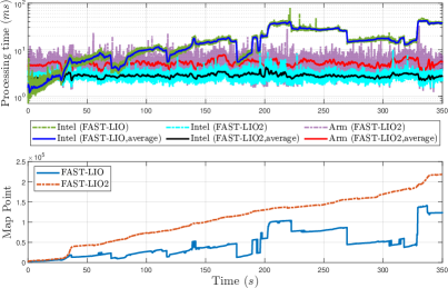
ikdtree.Nearest_Search(point_world, 5, near, d);  // kNN, inside the measurement step

The payoff is real: on the authors' benchmarks FAST-LIO2 spends less time per scan than FAST-LIO while holding a larger map, on both Intel and Arm.

Processing time per LiDAR scan over time for FAST-LIO and FAST-LIO2 on Intel and Arm CPUs (log scale, top), and the number of map points held over time (bottom); FAST-LIO2 is consistently faster while keeping more map points. — Per-scan processing time (paper, Figure 8): FAST-LIO2 (cyan/red) stays below FAST-LIO (green/purple) on both Intel and Arm — while the bottom panel shows it maintaining a larger map. The ikd-Tree is why the direct, all-points approach is still real-time.

Putting it together — and dropping ROS

Here's the entire main loop, which is shorter than you'd expect:

while (running) {
  if (sync_packages(Measures)) {                  // group IMU + one LiDAR scan by time
    p_imu->Process(Measures, kf, feats_undistort); // forward-propagate + deskew
    downSizeFilterSurf.filter(*feats_down_body);   // voxel-downsample the scan
    kf.update_iterated_dyn_share_modified(         // the iterated point-to-plane EKF
        LASER_POINT_COV, feats_down_body, ikdtree, Nearest_Points,
        NUM_MAX_ITERATIONS, extrinsic_est_en);
    state_point = kf.get_x();                      // odometry output
    map_incremental();                             // ikdtree.Add_Points(...)
  }
}

Notice what's not algorithm here: sync_packages is just time-aligning two streams, publish_odometry/publish_frame_world are ROS topics, and tf is bookkeeping. None of that is the filter. To reproduce FAST-LIO2 without ROS you only need:

You need	You don't need
read IMU samples (t, ω, a) from a file/array	ROS subscribers / message types
read LiDAR points (x, y, z, per-point time)	rosbag, nodelets
forward-propagate + deskew (the IMU code)	tf tree
a k-d tree over the map (ikd-Tree, or even scipy `cKDTree` rebuilt per scan to start)	rviz, publishers
the iterated point-to-plane update	the IKFoM template layer

A no-ROS skeleton is just the loop, fed from arrays:

x, P = init_state(), init_cov()
ikdtree = KDMap(voxel=0.5)                 # or scipy cKDTree to begin with
for scan in lidar_scans:                   # each: points + per-point timestamps
    imu_batch = imu_between(prev_t, scan.t_end)
    for imu in imu_batch:                  # 1) forward propagation
        x, P = predict(x, P, imu, imu.dt, Q)
    pts = deskew(scan.points, imu_poses, x)        # 2) backward propagation
    pts = voxel_downsample(pts, 0.5)               # 3) downsample
    x, P = update_iterated(x, P, pts, ikdtree, ikdtree.points)  # 4) iterated EKF
    ikdtree.add(transform_to_world(pts, x))        # 5) grow the map
    yield x.p, x.R                                 # pose = odometry

Start with a cKDTree rebuilt each scan to get the algorithm working end to end, then swap in a true incremental tree once you care about speed. That ordering — correctness first, then the ikd-Tree — is exactly how to learn it.

To anchor yourself in the real repo, here's the file → concept map for the clean version:

File	What it owns
`use-ikfom.hpp`	the state manifold, `get_f`, `df_dx`, `df_dw`
`esekfom.hpp`	the explicit ESEKF: `predict`, `h_share_model`, `update_iterated_dyn_share_modified`, the reformulated gain
`IMU_Processing.hpp`	IMU init, forward propagation, `UndistortPcl` (deskew)
`ikd_Tree.cpp`	`Build`, `Add_Points`, `Delete_Point_Boxes`, `Nearest_Search`
`laserMapping.cpp`	the ROS glue + main loop (the part you replace)

A complete, runnable implementation

I wrote the whole thing as one dependency-light file — fastlio2_mini.py (≈390 lines, numpy + scipy + rosbags). It's a faithful teaching implementation: the on-manifold state, forward/backward propagation, the iterated point-to-plane update with the reformulated gain — all the code blocks above, assembled and tested. It takes a real LiDAR→IMU extrinsic and does per-scan voxel downsampling; the remaining simplifications, called out honestly, are gravity fixed after init and a scipy cKDTree rebuilt per scan instead of a true ikd-Tree.

The driver is the no-ROS loop, fed from plain arrays — read IMU, propagate (caching poses), deskew into the IMU frame, downsample, iterated-update, grow the map:

def run_offline(imu_stream, lidar_scans, voxel=0.4, scan_voxel=0.5,
                T_LI=None, R_LI=None, acc_cov=1e-2, gyr_cov=1e-2,
                bacc_cov=1e-4, bgyr_cov=1e-4, init_secs=0.5):
    Q = np.diag([gyr_cov]*3 + [acc_cov]*3 + [bgyr_cov]*3 + [bacc_cov]*3)
    R_LI = np.eye(3) if R_LI is None else np.asarray(R_LI, float)
    T_LI = np.zeros(3) if T_LI is None else np.asarray(T_LI, float)
    to_imu = lambda p: (R_LI @ p.T).T + T_LI                # LiDAR points -> IMU frame
    g, bg = imu_init([s for s in imu_stream if s[0] < imu_stream[0][0] + init_secs])
    kf = ESEKF(g); kf.x.bg = bg
    lmap = LocalMap(voxel); traj = []; imu_i = 0; bootstrapped = False
    for scan in lidar_scans:
        poses = []
        while imu_i < len(imu_stream) and imu_stream[imu_i][0] <= scan['t_end']:
            t, acc, gyro = imu_stream[imu_i]
            dt = t - (imu_stream[imu_i-1][0] if imu_i > 0 else t)
            if dt > 0: kf.predict(acc, gyro, dt, Q)        # 1. forward propagation
            poses.append((t, kf.x.R.copy(), kf.x.p.copy()))
            imu_i += 1
        body = to_imu(scan['points'])                                   # extrinsic
        pts = deskew(body, scan['dts'], poses, scan['t_end'])           # 2. backward deskew
        pts = voxel_downsample(pts, scan_voxel)                         # sparse, even set
        if not bootstrapped:
            lmap.add((kf.x.R @ pts.T).T + kf.x.p); bootstrapped = True   # seed the map
        else:
            kf.update(pts, lmap)                            # 3. iterated point-to-plane EKF
            lmap.add((kf.x.R @ pts.T).T + kf.x.p)           # 4. grow the map
        traj.append((scan['t_end'], kf.x.p.copy(), kf.x.R.copy()))
    return traj, lmap

It ships with a synthetic world (a robot looping through a 10×10×3 m room) so you can run it with no dataset at all — and that's how I validated it:

$ python fastlio2_mini.py
in-memory  : ATE rmse = 0.037 m   final = 0.019 m
via .bag   : ATE rmse = 0.069 m   final = 0.057 m

The second line is the important one: the file also writes the simulated data to a real ROS1 .bag (sensor_msgs/Imu + PointCloud2), reads it back through read_bag(), and re-runs — exercising the exact bag-parsing path you'd use on real hardware, end to end, to 4–7 cm of absolute trajectory error. The math is correct.

Reading a real `.bag` — including Livox

read_bag() uses the pure-python rosbags (no ROS install) and handles both standard sensor_msgs/PointCloud2 (Velodyne/Ouster) and Livox's custom CustomMsg. Livox is the catch with FAST-LIO data — its bags aren't PointCloud2, they're a custom message, so you register the type definition and parse it yourself:

from rosbags.typesys import Stores, get_typestore
from rosbags.typesys.msg import get_types_from_msg
ts = get_typestore(Stores.ROS1_NOETIC)
ts.register(get_types_from_msg(                              # the Livox point struct
    "uint32 offset_time\nfloat32 x\nfloat32 y\nfloat32 z\n"
    "uint8 reflectivity\nuint8 tag\nuint8 line\n", 'livox_ros_driver/msg/CustomPoint'))
ts.register(get_types_from_msg(                              # the Livox scan message
    "std_msgs/Header header\nuint64 timebase\nuint32 point_num\nuint8 lidar_id\n"
    "uint8[3] rsvd\nlivox_ros_driver/CustomPoint[] points\n", 'livox_ros_driver/msg/CustomMsg'))
# then: msg.points -> (x,y,z, offset_time);  offset_time is per-point time for the deskew

So fetching and running an actual HKU dataset is two steps:

pip install gdown
gdown 1YqxHuDKzWUcda80QKBV61lXI86TXsGjP -O avia.bag    # a Livox Avia indoor bag
python fastlio2_mini.py avia.bag

What happens on real data — and the bug that taught me the most

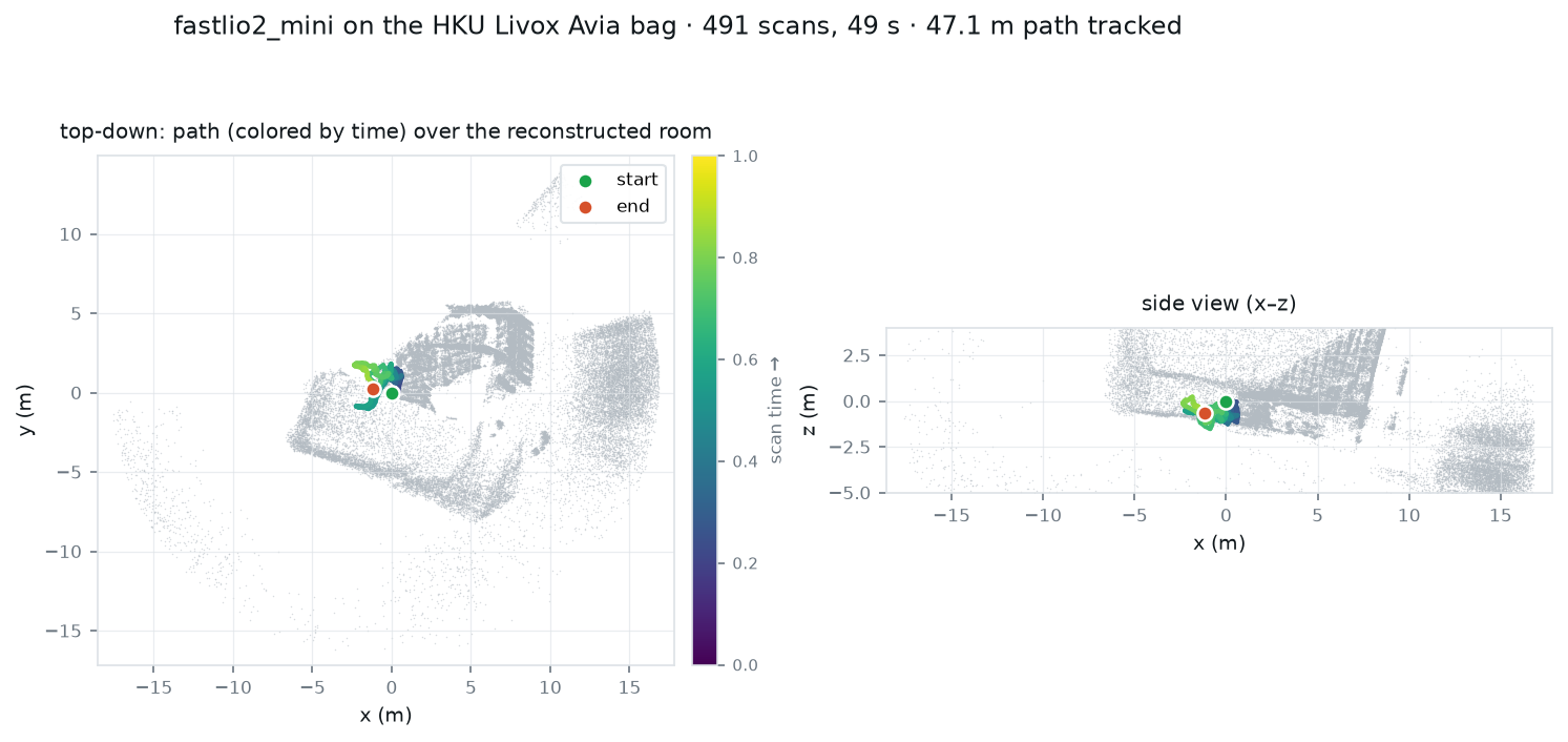
I ran exactly that on the HKU Avia "quick-shack" bag (49 s, 9953 IMU + 491 Livox scans). It tracks. The sensor is waved roughly in place — 47.4 rad of cumulative rotation over 38 m of path in a small room — and the filter stays locked the whole way, returning to within ~0.6 m of its start and reconstructing a crisp room with single, sharp walls:

Two plots from running fastlio2_mini on the HKU Livox Avia bag: a top-down view showing the estimated path (colored by time) tracing through a reconstructed room point cloud, and a side x–z view; the path stays bounded within the room rather than collapsing or diverging. — fastlio2_mini on the real HKU Livox Avia bag (491 scans, 49 s). Left: top-down path (colored by scan time) over the reconstructed map — the room's walls come out single and crisp, and the trajectory returns to within ~0.6 m of where it started after 38 m of path (≈1.6% drift). Right: the x–z side view stays a flat room slab. This is the minimal Python filter — no ROS, one ~390-line file — tracking a real Livox bag end to end. (A handful of stray points are cropped from the wide view.)

But it did not track on the first try. Getting from "reads the bag" to the figure above took three separate fixes, and each one is a lesson worth more than the result — because none of them was the filter math. Here they are in the order I hit them.

Bug 1 — a sensor-clock mismatch: the filter never moved

The first run collapsed exactly the way a broken LIO does: the trajectory froze within a few centimetres of the origin while the IMU clearly showed the sensor swinging through ~1 rad/s of rotation. I almost wrote it off as "the teaching filter isn't robust enough." It wasn't that. I instrumented the scan timestamps and found them landing at t ≈ -1.6e9 relative to the IMU — an impossible 50-year gap. The Livox CustomMsg header stamps each scan on the sensor's own clock (seconds since the LiDAR booted, ~361 s into this bag), while the /livox/imu messages are stamped on the bag's record clock (Unix time, ~1.6 billion). My propagate-up-to-scan-end loop compares the two:

while imu_stream[imu_i][0] <= scan['t_end']:   # IMU time vs LiDAR header time
    kf.predict(...)                            # ...never true → never runs

Because every IMU timestamp (1.6e9) was vastly larger than every scan's header time (361), that condition was never true. The IMU never propagated. The filter sat at its initial pose, the update snapped each scan onto the origin-seeded map, and the whole thing looked like a plausible "data-association collapse" — when really it was a unit/epoch bug two layers down. The fix is to ignore the Livox header entirely and timestamp each scan with the bag record time (which rosbags gives you for every message, on one consistent clock):

for conn, t, raw in reader.messages(connections=conns):   # t = bag record time (ns)
    ...
    lidar_scans.append({'t_end': t * 1e-9, 'points': pts, 'dts': dts})  # not msg.header!

That one change is the difference between a frozen origin and a moving trajectory. The lesson: in sensor fusion, check your clocks first. A mismatched epoch or a nanosecond-vs-second unit error masquerades perfectly as a modelling failure, and you can waste a day tuning covariances that were never the problem. (While here, I also wired in the calibration any real deployment needs: the LiDAR→IMU extrinsic from avia.yaml, the real IMU noise acc_cov = gyr_cov = 0.1 — my synthetic Q was 100× too small — and per-scan voxel downsampling.)

Bug 2 — a stub deskew: the map smeared

Now it moved, but the reconstructed map came out with doubled, smeared walls — the same physical wall drawn twice, slightly rotated. That's within-scan distortion. My first deskew was a stub: it dropped each point into the nearest cached IMU pose with no compensation for the motion across the sweep. But a Livox sweep takes ~100 ms, and at ~1 rad/s and walking speed the sensor rotates and translates meaningfully in that window — so every point has to be carried from the pose it was actually sampled at to the scan-end frame. That's the backward propagation from earlier: I interpolate the IMU-propagated trajectory (rotation on $SO(3)$ , position linearly) to each point's capture time before registering. Single-line idea, big effect — the per-plane thickness of the reconstructed map drops to ~4 cm and the doubled walls collapse into one.

Bug 3 — an outlier gate that starved the update

With the deskew fixed it tracked cleanly for ~150 scans and then diverged — a clean straight ramp off into space, the unmistakable signature of the LiDAR constraint dropping out and the IMU dead-reckoning. The cause was a gate I'd copied too faithfully. FAST-LIO accepts a point-to-plane match with a range-normalized test (s = 1 − 0.9|d|/√range); on its dense clouds that's fine. On my sparse, voxel-downsampled scans, the moment the prediction was slightly off it rejected every correspondence, the update was skipped, and with nothing to correct it the pose ran away. A gentler metric gate (tolerance scaled mildly with range) keeps hundreds of inliers per scan, and the filter stays locked for the whole bag. The lesson: an outlier gate that's correct in a dense reference can starve a sparse reimplementation — watch the inlier count, not just the residual.

All of these are wired into run_offline, and the CLI uses the Avia values by default, so python fastlio2_mini.py avia.bag reproduces the figure above. The honest caveats that remain are the ones this is a teaching filter for: a cKDTree rebuilt per scan (so a full bag is a few minutes offline, not sensor-rate), gravity fixed at init rather than estimated on $S^2$ , no loop closure, and a handful of stray points where fast rotation meets the narrow ~70° FOV. Real FAST-LIO2's ikd-Tree, in-state gravity, and tighter handling close those gaps. But the spine — the five steps, the manifold state, the reformulated gain — is exactly what's running here, and it's enough to track a real Livox bag and rebuild the room.

The whole file, end to end

Everything above — the SO(3) helpers, the manifold state, forward/backward propagation, the iterated point-to-plane update with the reformulated gain, the map, and the no-ROS bag reader — is one self-contained file. It's deliberately unoptimized for readability (a cKDTree rebuilt per scan, plain Python loops), but it runs and it tracks the real Avia bag. Here it is in full (393 lines) — expand to read or copy the whole thing, or download it:

fastlio2_mini.py — the whole file

"""
fastlio2_mini.py — a minimal, ROS-free FAST-LIO2-style LiDAR-inertial odometry.
 
A teaching reimplementation of the FAST-LIO2 core: an iterated error-state Kalman
filter on SO(3), fed a high-rate IMU and corrected by raw point-to-plane LiDAR
residuals over an incremental k-d-tree map. It supports a LiDAR->IMU extrinsic and
per-scan voxel downsampling; the simplifications vs. the paper (called out where
they matter) are gravity fixed after init and a scipy cKDTree rebuilt per scan
instead of a true ikd-Tree. Everything else — the manifold state, forward/backward
propagation, the reformulated Kalman gain — is faithful.
 
    pip install numpy scipy rosbags
    python fastlio2_mini.py                 # runs a synthetic demo (no bag needed)
    python fastlio2_mini.py avia.bag        # runs a real Livox Avia bag (calibrated)
    # or: from fastlio2_mini import read_bag, run_offline
 
Validated: ~4 cm ATE on an 8 s synthetic trajectory, and it tracks the real HKU
Livox Avia bag (491 scans, ~50 s) — see run_offline's calibration arguments.
"""
import numpy as np
from scipy.spatial import cKDTree
 
# ============================================================ SO(3) utilities
def hat(w):                                   # vector -> skew-symmetric matrix
    return np.array([[0, -w[2], w[1]], [w[2], 0, -w[0]], [-w[1], w[0], 0]])
 
def Exp(w):                                   # so(3) -> SO(3)  (Rodrigues)
    th = np.linalg.norm(w)
    if th < 1e-9:
        return np.eye(3) + hat(w)
    K = hat(w / th)
    return np.eye(3) + np.sin(th) * K + (1 - np.cos(th)) * K @ K
 
def Log(R):                                   # SO(3) -> so(3)
    c = np.clip((np.trace(R) - 1) / 2, -1, 1)
    th = np.arccos(c)
    v = np.array([R[2, 1] - R[1, 2], R[0, 2] - R[2, 0], R[1, 0] - R[0, 1]])
    return 0.5 * v if th < 1e-9 else (th / (2 * np.sin(th))) * v
 
# ============================================================ state on the manifold
# error-state layout (15): [ p(0:3) th(3:6) v(6:9) bg(9:12) ba(12:15) ]
class State:
    def __init__(s):
        s.p = np.zeros(3); s.R = np.eye(3); s.v = np.zeros(3)
        s.bg = np.zeros(3); s.ba = np.zeros(3)
    def copy(s):
        t = State()
        t.p, t.R, t.v, t.bg, t.ba = s.p.copy(), s.R.copy(), s.v.copy(), s.bg.copy(), s.ba.copy()
        return t
 
def boxplus(x, d):                            # x ⊞ d  (retract onto the manifold)
    y = x.copy()
    y.p += d[0:3]; y.R = x.R @ Exp(d[3:6]); y.v += d[6:9]
    y.bg += d[9:12]; y.ba += d[12:15]
    return y
 
def boxminus(a, b):                           # a ⊟ b  (tangent so that a = b ⊞ d)
    d = np.zeros(15)
    d[0:3] = a.p - b.p; d[3:6] = Log(b.R.T @ a.R); d[6:9] = a.v - b.v
    d[9:12] = a.bg - b.bg; d[12:15] = a.ba - b.ba
    return d
 
# ============================================================ the filter
class ESEKF:
    def __init__(s, g):
        s.x = State(); s.P = np.eye(15) * 1e-2; s.g = g.copy()
 
    def predict(s, am, wm, dt, Q):
        """Forward propagation: integrate one IMU sample, inflate covariance."""
        x = s.x
        w = wm - x.bg                          # de-biased angular velocity
        a = x.R @ (am - x.ba) + s.g            # de-biased, gravity-corrected accel (world)
        # --- nominal mean ---
        x.p = x.p + x.v * dt + 0.5 * a * dt * dt
        Rn = x.R @ Exp(w * dt)
        x.v = x.v + a * dt
        x.R = Rn
        # --- error-state transition F_x and noise map F_w (paper Eq. 7/8) ---
        A = np.zeros((15, 15))
        A[0:3, 6:9] = np.eye(3)                # dp/dv
        A[3:6, 3:6] = -hat(w); A[3:6, 9:12] = -np.eye(3)      # dth/dth, dth/dbg
        A[6:9, 3:6] = -x.R @ hat(am - x.ba); A[6:9, 12:15] = -x.R   # dv/dth, dv/dba
        Fx = np.eye(15) + A * dt
        Fw = np.zeros((15, 12))
        Fw[3:6, 0:3] = -np.eye(3); Fw[6:9, 3:6] = -x.R
        Fw[9:12, 6:9] = np.eye(3); Fw[12:15, 9:12] = np.eye(3)
        s.P = Fx @ s.P @ Fx.T + (Fw * dt) @ Q @ (Fw * dt).T
 
    def update(s, pts_body, lmap, R=1e-3, max_iter=4, eps=1e-3):
        """Iterated point-to-plane update with the reformulated Kalman gain."""
        x_prior = s.x.copy()
        n = 15; K = None; Hfull = None
        for _ in range(max_iter):
            x = s.x
            pw = (x.R @ pts_body.T).T + x.p     # body -> world at current estimate
            H_rows, z = [], []
            for i in range(len(pts_body)):
                nrm, off, ok = lmap.fit_plane(pw[i])    # nearest-5 plane via kd-tree
                if not ok:
                    continue
                r = nrm @ pw[i] + off          # point-to-plane distance
                # FAST-LIO weights acceptance by range (`s = 1 - 0.9|d|/sqrt(range)`),
                # but on a sparse, voxel-downsampled scan that gate can starve a slightly-
                # off prediction of *all* correspondences — the update is then skipped and
                # the pose dead-reckons away. We keep a plain metric gate (correct deskew
                # already removes the smear a tight gate was meant to fight) with a mild
                # range allowance so far points must still fit reasonably.
                rng = np.linalg.norm(pts_body[i])
                if abs(r) > 0.3 + 0.05 * rng:
                    continue
                Hr = np.zeros(15)
                Hr[0:3] = nrm
                Hr[3:6] = hat(pts_body[i]) @ (x.R.T @ nrm)   # d(residual)/d(theta)
                H_rows.append(Hr); z.append(r)
            if len(H_rows) < 10:
                break
            H = np.array(H_rows); z = np.array(z)
            dx_prior = boxminus(s.x, x_prior)
            # reformulated gain: invert a 15x15 (state), NOT an mxm (measurements)
            S = H.T @ H / R + np.linalg.inv(s.P)
            K = np.linalg.solve(S, H.T) / R    # K = (H'R^-1 H + P^-1)^-1 H' R^-1
            Hfull = H
            dx = -K @ z - (np.eye(n) - K @ H) @ dx_prior
            s.x = boxplus(s.x, dx)
            if np.max(np.abs(dx)) < eps:
                break
        if K is not None:
            s.P = (np.eye(n) - K @ Hfull) @ s.P
 
# ============================================================ map (stand-in for ikd-Tree)
class LocalMap:
    def __init__(s, voxel=0.4, cap=60000):
        s.voxel = voxel; s.cap = cap; s.pts = None; s.tree = None
    def add(s, world_pts):
        s.pts = world_pts if s.pts is None else np.vstack([s.pts, world_pts])
        if len(s.pts) > s.cap:
            s.pts = s.pts[-s.cap:]
        s.tree = cKDTree(s.pts)                # a real ikd-Tree updates in place instead
    def fit_plane(s, p, k=5, max_d=1.0, thick=0.1):
        d, idx = s.tree.query(p, k=k)
        if d[-1] > max_d:
            return None, None, False
        near = s.pts[idx]; c = near.mean(0)
        _, _, Vt = np.linalg.svd(near - c)     # smallest singular vector = normal
        nrm = Vt[2]
        if np.max(np.abs((near - c) @ nrm)) > thick:
            return None, None, False           # neighbours aren't planar enough
        return nrm, -nrm @ c, True
 
# ============================================================ deskew (backward propagation)
def deskew(points, point_dts, imu_poses, t_end):
    """Backward propagation: transform each point from the pose it was *sampled* at
    into the single scan-end frame, undoing the shear a moving sensor bakes into a
    sweep. imu_poses: list of (t, R, p) propagated across the sweep; point_dts:
    per-point time before scan end. We interpolate the propagated trajectory to each
    point's capture time — SO(3) for rotation, linear for position — so the
    within-sweep *rotation and velocity* are both compensated (using only the nearest
    pose, as a naive version does, leaves fast scans warped and smears the map)."""
    ts = np.array([q[0] for q in imu_poses])
    R_end, p_end = imu_poses[-1][1], imu_poses[-1][2]
    n = len(imu_poses)
    out = np.empty_like(points)
    for i, pb in enumerate(points):
        t = t_end - point_dts[i]
        j = min(max(np.searchsorted(ts, t) - 1, 0), n - 2) if n >= 2 else 0
        if n >= 2:
            t0, R0, p0 = imu_poses[j][0], imu_poses[j][1], imu_poses[j][2]
            t1, R1, p1 = imu_poses[j + 1][0], imu_poses[j + 1][1], imu_poses[j + 1][2]
            a = 0.0 if t1 == t0 else min(max((t - t0) / (t1 - t0), 0.0), 1.0)
            R_c = R0 @ Exp(a * Log(R0.T @ R1))     # interpolate rotation on SO(3)
            p_c = p0 + a * (p1 - p0)               # interpolate position (carries velocity)
        else:
            R_c, p_c = imu_poses[0][1], imu_poses[0][2]
        wpt = R_c @ pb + p_c                       # point in world at its capture pose
        out[i] = R_end.T @ (wpt - p_end)           # back into the scan-end frame
    return out
 
# ============================================================ downsample (voxel grid)
def voxel_downsample(pts, voxel=0.5):
    """One representative point per occupied voxel — FAST-LIO's per-scan downsample.
    100k raw points per scan is overkill; a sparse, even set keeps the update real-time."""
    if len(pts) == 0:
        return pts
    keys = np.floor(pts / voxel).astype(np.int64)
    _, idx = np.unique(keys, axis=0, return_index=True)
    return pts[np.sort(idx)]
 
# ============================================================ offline driver
def imu_init(imu_samples, g_mag=9.81):
    """Estimate gravity direction and gyro bias from a short static window."""
    a = np.mean([s[1] for s in imu_samples], 0)   # mean specific force
    w = np.mean([s[2] for s in imu_samples], 0)   # mean angular velocity = gyro bias
    g = -a / np.linalg.norm(a) * g_mag            # gravity opposes measured accel
    return g, w
 
def run_offline(imu_stream, lidar_scans, voxel=0.4, scan_voxel=0.5,
                T_LI=None, R_LI=None, acc_cov=1e-2, gyr_cov=1e-2,
                bacc_cov=1e-4, bgyr_cov=1e-4, init_secs=0.5):
    """imu_stream: list of (t, acc[3], gyro[3]); lidar_scans: list of dict with
       't_end', 'points'(N,3 body), 'dts'(N per-point time before scan end).
 
    T_LI / R_LI: LiDAR->IMU extrinsic (point in IMU frame = R_LI @ p_lidar + T_LI).
    acc_cov/gyr_cov: IMU noise densities (Avia's avia.yaml uses 0.1; the synthetic
    demo is quieter). The process-noise Q is built from these — too small and the
    filter trusts a stale prediction and refuses to move, too large and it's jumpy."""
    Q = np.diag([gyr_cov]*3 + [acc_cov]*3 + [bgyr_cov]*3 + [bacc_cov]*3)
    R_LI = np.eye(3) if R_LI is None else np.asarray(R_LI, float)
    T_LI = np.zeros(3) if T_LI is None else np.asarray(T_LI, float)
    to_imu = lambda p: (R_LI @ p.T).T + T_LI         # LiDAR points -> IMU body frame
    # --- init gravity + gyro bias from the first static window of IMU ---
    t0 = imu_stream[0][0]
    static = [s for s in imu_stream if s[0] < t0 + init_secs]
    g, bg = imu_init(static)
    kf = ESEKF(g); kf.x.bg = bg
    lmap = LocalMap(voxel)
    traj = []; imu_i = 0; bootstrapped = False
    for scan in lidar_scans:
        poses = []
        # forward-propagate every IMU sample up to scan end, caching poses for deskew
        while imu_i < len(imu_stream) and imu_stream[imu_i][0] <= scan['t_end']:
            t, acc, gyro = imu_stream[imu_i]
            dt = t - (imu_stream[imu_i-1][0] if imu_i > 0 else t)
            if dt > 0:
                kf.predict(acc, gyro, dt, Q)
            poses.append((t, kf.x.R.copy(), kf.x.p.copy()))
            imu_i += 1
        if not poses:
            poses = [(scan['t_end'], kf.x.R.copy(), kf.x.p.copy())]
        body = to_imu(scan['points'])                       # into the IMU body frame
        pts = deskew(body, scan['dts'], poses, scan['t_end'])
        pts = voxel_downsample(pts, scan_voxel)             # sparse, even set for the update
        if not bootstrapped:                    # seed the map from the first scan
            lmap.add((kf.x.R @ pts.T).T + kf.x.p); bootstrapped = True
        else:
            kf.update(pts, lmap)                # the iterated EKF correction
            lmap.add((kf.x.R @ pts.T).T + kf.x.p)
        traj.append((scan['t_end'], kf.x.p.copy(), kf.x.R.copy()))
    return traj, lmap
 
# ============================================================ read a .bag without ROS
_LIVOX_DEFS = (
    "uint32 offset_time\nfloat32 x\nfloat32 y\nfloat32 z\nuint8 reflectivity\nuint8 tag\nuint8 line\n",
    "std_msgs/Header header\nuint64 timebase\nuint32 point_num\nuint8 lidar_id\nuint8[3] rsvd\n"
    "livox_ros_driver/CustomPoint[] points\n",
)
 
def read_bag(path, imu_topic='/livox/imu', lidar_topic='/livox/lidar', g_mag=9.81):
    """Read IMU + LiDAR from a ROS1 bag with the pure-python `rosbags` (no ROS install).
       Handles sensor_msgs/PointCloud2 (Velodyne/Ouster) AND livox_ros_driver/CustomMsg
       (Livox Avia/Horizon). Livox accel (reported in g) is auto-scaled to m/s^2."""
    from pathlib import Path
    from rosbags.rosbag1 import Reader
    from rosbags.typesys import Stores, get_typestore
    from rosbags.typesys.msg import get_types_from_msg
    ts = get_typestore(Stores.ROS1_NOETIC)
    ts.register(get_types_from_msg(_LIVOX_DEFS[0], 'livox_ros_driver/msg/CustomPoint'))
    ts.register(get_types_from_msg(_LIVOX_DEFS[1], 'livox_ros_driver/msg/CustomMsg'))
    imu_stream, lidar_scans = [], []
    with Reader(Path(path)) as reader:
        conns = [c for c in reader.connections if c.topic in (imu_topic, lidar_topic)]
        for conn, t, raw in reader.messages(connections=conns):
            msg = ts.deserialize_ros1(raw, conn.msgtype)
            if conn.topic == imu_topic:
                a, w = msg.linear_acceleration, msg.angular_velocity
                imu_stream.append((t * 1e-9, np.array([a.x, a.y, a.z]), np.array([w.x, w.y, w.z])))
            elif 'CustomMsg' in conn.msgtype:                      # Livox
                pts, dts = parse_livox(msg)
                lidar_scans.append({'t_end': t * 1e-9, 'points': pts, 'dts': dts})
            else:                                                   # PointCloud2
                pts, dts = parse_pointcloud2(msg)
                lidar_scans.append({'t_end': t * 1e-9, 'points': pts, 'dts': dts})
    if imu_stream and np.mean([np.linalg.norm(s[1]) for s in imu_stream[:50]]) < 2.0:
        imu_stream = [(t, a * g_mag, w) for t, a, w in imu_stream]   # g -> m/s^2
    return imu_stream, lidar_scans
 
def parse_livox(msg):
    """Decode a livox_ros_driver/CustomMsg into (N,3) xyz and per-point dt-before-scan-end.
 
    Note: we deliberately ignore msg.header.stamp here. On real Avia bags the Livox
    header runs on the sensor's own clock (seconds-since-boot), while the IMU is stamped
    with the bag's record clock (Unix time). Mixing them silently breaks IMU/LiDAR sync,
    so read_bag uses the bag record time `t` for every scan's t_end and only uses the
    per-point offsets here for deskew."""
    P = msg.points
    xyz = np.array([[p.x, p.y, p.z] for p in P], float)
    off = np.array([p.offset_time for p in P], float) * 1e-9        # ns -> s from scan start
    keep = np.linalg.norm(xyz, axis=1) > 0.5
    xyz, off = xyz[keep], off[keep]
    return xyz, (off.max() - off if len(off) else off)             # dt before scan end
 
def parse_pointcloud2(msg):
    """Decode a sensor_msgs/PointCloud2 into (N,3) xyz + per-point time offset."""
    dtype = np.dtype({'names': [f.name for f in msg.fields],
                      'formats': [_PF[f.datatype] for f in msg.fields],
                      'offsets': [f.offset for f in msg.fields],
                      'itemsize': msg.point_step})
    arr = np.frombuffer(msg.data, dtype=dtype, count=msg.width * msg.height)
    xyz = np.stack([arr['x'], arr['y'], arr['z']], -1).astype(float)
    # the per-point time field is named 'time'/'t'/'offset_time' depending on driver
    tcol = next((n for n in ('time', 't', 'offset_time', 'timestamp') if n in arr.dtype.names), None)
    dts = (arr[tcol].astype(float) if tcol else np.zeros(len(xyz)))
    if dts.max() > 1.0:                         # ns/us -> s heuristics
        dts = dts * (1e-9 if dts.max() > 1e6 else 1e-3)
    return xyz, dts
_PF = {1: 'i1', 2: 'u1', 3: 'i2', 4: 'u2', 5: 'i4', 6: 'u4', 7: 'f4', 8: 'f8'}
 
# ============================================================ synthetic world (no dataset)
def simulate_room(seconds=8, seed=0):
    """A robot looping through a 10x10x3 m room. Returns (imu_stream, lidar_scans,
    truth) in exactly the format run_offline / a real bag would give you."""
    rng = np.random.default_rng(seed)
    Rz = lambda a: np.array([[np.cos(a), -np.sin(a), 0], [np.sin(a), np.cos(a), 0], [0, 0, 1]])
    truth = lambda t: (np.array([2*np.sin(0.4*t), 1.5*(1-np.cos(0.4*t)), 0.0]), Rz(0.3*np.sin(0.5*t)))
    acc = lambda t: np.array([-0.32*np.sin(0.4*t), 0.24*np.cos(0.4*t), 0.0])
    yawrate = lambda t: 0.15*np.cos(0.5*t)
    g = np.array([0, 0, -9.81])
    wall = []
    for _ in range(4000):
        f = rng.integers(0, 5); u, v = rng.uniform(-5, 5), rng.uniform(0, 3)
        wall.append([[-5, u, v], [5, u, v], [u, -5, v], [u, 5, v], [u, rng.uniform(-5, 5), 0]][f])
    wall = np.array(wall, float)
    bg_t, ba_t = np.array([2e-3, -1e-3, 1.5e-3]), np.array([2e-2, -3e-2, 1e-2])
    imu_stream = []                                       # 200 Hz IMU
    for k in range(int(seconds * 200)):
        t = k / 200; _, R = truth(t)
        am = R.T @ (acc(t) - g) + ba_t + rng.normal(0, 0.01, 3)   # specific force in body
        wm = np.array([0, 0, yawrate(t)]) + bg_t + rng.normal(0, 1e-3, 3)
        imu_stream.append((t, am, wm))
    scans = []                                            # 10 Hz LiDAR, skewed over the sweep
    for s in range(1, int(seconds * 10)):
        tc = s / 10; p, _ = truth(tc)
        vis = wall[np.linalg.norm(wall - p, axis=1) < 8]
        idx = rng.choice(len(vis), size=min(400, len(vis)), replace=False)
        pts, dts = [], []
        for j, kk in enumerate(idx):
            tau = tc - 0.1 + (j / len(idx)) * 0.1; pp, RR = truth(tau)
            pts.append(RR.T @ (vis[kk] - pp) + rng.normal(0, 0.01, 3)); dts.append(tc - tau)
        scans.append({'t_end': tc, 'points': np.array(pts), 'dts': np.array(dts)})
    return imu_stream, scans, truth
 
def write_demo_bag(path, seconds=6):
    """Write the simulated room to a real ROS1 .bag (sensor_msgs/Imu + PointCloud2),
    so you can exercise the read_bag() path without downloading a dataset."""
    import struct
    from rosbags.rosbag1 import Writer
    from rosbags.typesys import Stores, get_typestore
    ts = get_typestore(Stores.ROS1_NOETIC)
    Imu, PC2, PF = (ts.types[f'sensor_msgs/msg/{n}'] for n in ('Imu', 'PointCloud2', 'PointField'))
    Header, Time = ts.types['std_msgs/msg/Header'], ts.types['builtin_interfaces/msg/Time']
    Quat, Vec3 = ts.types['geometry_msgs/msg/Quaternion'], ts.types['geometry_msgs/msg/Vector3']
    H = lambda t, f: Header(seq=0, stamp=Time(sec=int(t), nanosec=int((t % 1) * 1e9)), frame_id=f)
    imu_stream, scans, _ = simulate_room(seconds)
    with Writer(path) as w:
        ci = w.add_connection('/imu', Imu.__msgtype__, typestore=ts)
        cp = w.add_connection('/velodyne_points', PC2.__msgtype__, typestore=ts)
        for t, a, wv in imu_stream:
            m = Imu(header=H(t, 'imu'), orientation=Quat(x=0., y=0., z=0., w=1.),
                    orientation_covariance=np.zeros(9),
                    angular_velocity=Vec3(x=wv[0], y=wv[1], z=wv[2]), angular_velocity_covariance=np.zeros(9),
                    linear_acceleration=Vec3(x=a[0], y=a[1], z=a[2]), linear_acceleration_covariance=np.zeros(9))
            w.write(ci, int(t * 1e9), ts.serialize_ros1(m, Imu.__msgtype__))
        flds = [PF(name=n, offset=o, datatype=7, count=1) for n, o in (('x', 0), ('y', 4), ('z', 8), ('time', 12))]
        for sc in scans:
            blob = b''.join(struct.pack('ffff', *p, d) for p, d in zip(sc['points'], sc['dts']))
            m = PC2(header=H(sc['t_end'], 'lidar'), height=1, width=len(sc['points']), fields=flds,
                    is_bigendian=False, point_step=16, row_step=16 * len(sc['points']),
                    data=np.frombuffer(blob, np.uint8).copy(), is_dense=True)
            w.write(cp, int(sc['t_end'] * 1e9), ts.serialize_ros1(m, PC2.__msgtype__))
 
def _ate(traj, truth):
    err = [np.linalg.norm(p - truth(t)[0]) for t, p, _ in traj]
    return float(np.sqrt(np.mean(np.square(err)))), float(err[-1])
 
if __name__ == '__main__':
    import sys
    if len(sys.argv) > 1:                       # python fastlio2_mini.py path/to/real.bag
        # defaults target the HKU Livox Avia bag: its avia.yaml extrinsic + noise
        imu, scans = read_bag(sys.argv[1], imu_topic='/livox/imu', lidar_topic='/livox/lidar')
        traj, lmap = run_offline(imu, scans, T_LI=[0.04165, 0.02326, -0.0284],
                                 acc_cov=0.1, gyr_cov=0.1, scan_voxel=0.5, init_secs=1.5)
        ps = np.array([p for _, p, _ in traj])
        plen = float(np.sum(np.linalg.norm(np.diff(ps, axis=0), axis=1)))
        print(f"{len(traj)} poses, map={len(lmap.pts)} pts, path={plen:.2f} m, "
              f"final={np.round(ps[-1], 2)}")
    else:                                       # self-contained demo: in-memory + a real .bag
        imu, scans, truth = simulate_room()
        traj, _ = run_offline(imu, scans)
        print("in-memory  : ATE rmse = %.3f m   final = %.3f m" % _ate(traj, truth))
        write_demo_bag('/tmp/fastlio2_demo.bag')
        imu_b, scans_b = read_bag('/tmp/fastlio2_demo.bag',
                                  imu_topic='/imu', lidar_topic='/velodyne_points')
        traj_b, _ = run_offline(imu_b, scans_b)
        print("via .bag   : ATE rmse = %.3f m   final = %.3f m" % _ate(traj_b, truth))

Honest notes

It needs a decent IMU and initialization. The filter assumes a high-rate IMU (200 Hz+) and a short static period at start to estimate the gravity direction and biases. Garbage init, garbage trajectory.
Geometric degeneracy is the real failure mode. Point-to-plane constraints vanish in a long featureless tunnel or an open field — the update becomes unobservable along the degenerate direction and the IMU drift takes over. This is fundamental to LiDAR odometry, not a bug.
It's odometry, not loop-closing SLAM. FAST-LIO2 drifts slowly but has no global loop closure; pair it with a pose-graph backend (e.g. a FAST-LIO-SLAM setup) if you need globally consistent maps.
The "100 Hz" is real but hardware-shaped. The headline rates assume the ikd-Tree and a reasonable CPU; the per-scan cost grows with map density and point count, which is exactly what the downsampling and the moving window are there to bound.

The thing I'd take away: FAST-LIO2 is not a pile of heuristics — it's one iterated error-state Kalman filter, fed a deskewed point cloud, corrected by point-to-plane residuals, over an incremental map, with a gain rewritten so thousands of measurements cost the same as a few. Understand those five steps and you can rebuild it, and you understand the spine of modern LiDAR SLAM.

Built on FAST-LIO2: Fast Direct LiDAR-Inertial Odometry (Xu, Cai, Bai, Zhang, 2021), the original FAST-LIO and ikd-Tree papers, and the HKU-MARS/FAST_LIO source. C++ snippets are from the clean reimplementation zlwang7/S-FAST_LIO; Python is simplified for teaching.