SOG: a Gaussian splat scene as spatially-ordered WebP images

mdjsonmcpcopy↗ai

2026-10-02 · 18 min · 3d · gaussian-splatting · quantization · webgpu · explainer

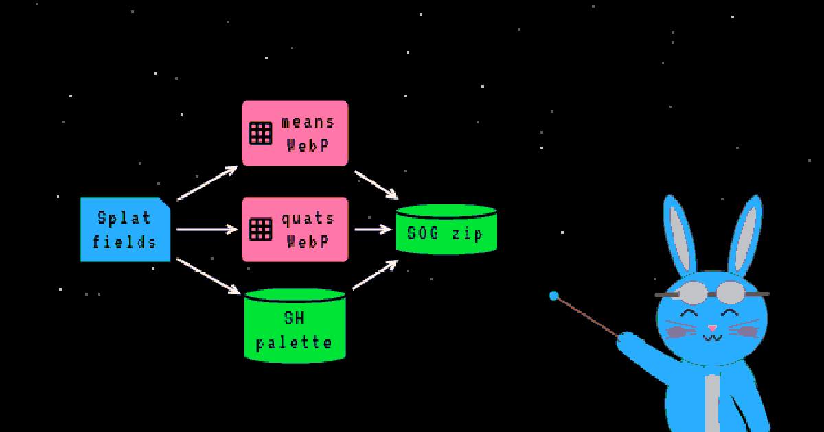
A 3D Gaussian Splatting scene is a point cloud where every point is a fuzzy, oriented, coloured ellipsoid. Train one on a few hundred photos and you get millions of them. They render beautifully and in real time — and then you have to move the file, and the file is enormous.

Here is exactly how enormous. I pulled the example dataset the ColmapView author published to Hugging Face — the Mip-NeRF 360 bicycle scene, trained to 30,000 iterations — and read the two splat files it ships. Same scene, same 5,000,000 Gaussians, two encodings:

That is 1.18 GB versus 65 MB, an 18.18x shrink (measured: the two files, divided). The PLY is the standard output of the original 3DGS trainer; the SOG is PlayCanvas's open SOG format — Spatially Ordered Gaussians — written by SplatTransform and read, here, by ColmapView 15.

expand

The question worth answering is not that SOG is smaller — every compressed splat format claims that — but where the other seventeen-eighteenths go, field by field, and how much of the win is clever quantization versus the "spatially ordered" part of the name. So I took the real file apart. The short version: quantization does most of the work, dropping 248 bytes to about 19; the spatial ordering plus WebP does the rest, 19 down to the measured 13.64. The longer version is the interesting one, because the spatial ordering leaves a visible fingerprint in the file.

What one splat stores, and why PLY is big

A single Gaussian in a 3DGS scene is defined by a handful of parameters:

• a position $\mu \in \mathbb{R}^3$ — where the ellipsoid sits;
• a rotation as a unit quaternion $q = (w, x, y, z)$ — how it is turned;
• an anisotropic scale $s \in \mathbb{R}^3$ — its size along its own three axes;
• an opacity $\alpha$ — how solidly it occludes;
• a colour expressed as spherical-harmonic coefficients, so the colour can change with viewing angle (specular highlights, sheen). Degree 0 is one RGB triple (the flat, view-independent colour); degrees 1 through 3 add 15 more coefficients per channel, 45 floats, for the view-dependent part.

The reference 3DGS trainer dumps all of that to a binary PLY as float32, one vertex per splat. I read the header of the real file to be sure of the layout:

element vertex 5000000
property float x  y  z                 # position            3
property float nx ny nz                # normals             3  (always zero)
property float f_dc_0 f_dc_1 f_dc_2    # SH degree 0 (DC)    3
property float f_rest_0 ... f_rest_44  # SH degrees 1-3      45
property float opacity                 # opacity             1
property float scale_0 scale_1 scale_2 # scale               3
property float rot_0 rot_1 rot_2 rot_3 # quaternion          4

That is 62 float32 properties = 248 bytes per splat (measured: the file is exactly 5,000,000 x 248 + 1,532 header bytes). Two things jump out. The nx, ny, nz normals are vestigial — 3DGS does not use surface normals, the trainer writes them as zeros, and they still cost 12 bytes a splat. And the 45 f_rest floats — the higher-order spherical harmonics — are 180 bytes, over 70% of every splat, spent on the angle-dependent sheen that a viewer three metres away can barely see. A format that wants to be small has to go after those 45 floats first.

The SOG idea: don't write a codec, reuse WebP

The move SOG makes is to stop thinking of a splat scene as a list of structs and start thinking of each attribute as an image. Lay the splats out in a rectangle — splat i goes to pixel (i % W, floor(i / W)), row-major — and then every attribute becomes a texture with one pixel per splat: a positions image, a scales image, a quaternion image, a colour image. Quantize each attribute down to 8 or 16 bits so it fits in image channels, and save the textures as lossless WebP.

Why WebP? Because you get a mature, ubiquitous, GPU-adjacent entropy coder for free — every browser decodes it — and because the data you are handing it is a 2D image of spatially-coherent scene attributes, which is exactly what image predictors are built to compress. The container is deliberately boring:

scene.sog  (a zip)
├── meta.json          # version, count, per-axis ranges, codebooks
├── means_l.webp       # positions, low 8 bits  (RGB)
├── means_u.webp       # positions, high 8 bits (RGB)
├── scales.webp        # 3 codebook indices     (RGB)
├── quats.webp         # smallest-three         (RGBA)
├── sh0.webp           # DC colour + opacity    (RGBA)
├── shN_centroids.webp # SH palette             (RGB)
└── shN_labels.webp    # SH palette index       (RG)

The same files can live unzipped in a directory (nicer for authoring) or be bundled into a single .sog zip (nicer for shipping); the reader accepts both. The real bicycle bundle is this exact set — eight entries, which I read straight out of the zip's central directory.

Field by field: where 248 bytes become 13.64

Take the attributes in turn. Every number below is from the real file, and I have labelled each one.

Position — 12 B to 6 B of raw pixels. Each axis gets 16 bits, split across two images: the high byte of x, y, z goes into the RGB of means_u.webp, the low byte into means_l.webp. The values are stored in a symmetric (signed) log domain and dequantized through per-axis mins/maxs carried in meta.json (reported, SOG spec) — the log keeps precision high near the origin, where the scene is dense, without clipping the far splats. Six raw bytes, half of PLY's twelve, before any compression.

Rotation — 16 B to 4 B. A unit quaternion has only three degrees of freedom: $w^2 + x^2 + y^2 + z^2 = 1$, so once you know three components you can reconstruct the fourth. SOG uses the classic smallest-three trick: drop the component with the largest magnitude (it reconstructs as $\sqrt{1 - a^2 - b^2 - c^2}$, taken positive), store the other three at 8 bits each over $[-\tfrac{\sqrt2}{2}, +\tfrac{\sqrt2}{2}]$, and record which of the four was dropped in a 2-bit "mode". That is 26 bits of information — three 8-bit components plus a 2-bit tag — packed into the 32-bit RGBA of quats.webp, where the alpha channel carries the mode as a value in 252..255 (reported, SOG spec). Sixteen float bytes down to four.

Scale — 12 B to 3 B. The three log-scales are quantized to 8-bit indices into a 256-entry codebook of log-domain values stored in meta.json; the reader does exp() on the looked-up value to recover a linear size. One byte per axis, into the RGB of scales.webp.

Base colour + opacity — 16 B to 4 B. The DC colour (three floats) becomes three 8-bit indices into a 256-float colour codebook; the opacity becomes a single 8-bit value, opacity = A / 255. Both ride in one image, sh0.webp, colour in RGB and opacity in alpha.

The higher-order SH — 180 B to 2 B. This is the whole game. Instead of storing 45 floats per splat, SOG vector-quantizes the entire 45-dimensional SH-rest vector into a shared palette of up to 65,536 centroids, and stores one 16-bit index per splat in shN_labels.webp (index = R + (G << 8)). The palette itself lives in shN_centroids.webp, and in the real file it holds exactly 65,536 entries (measured, from meta.json: shN.count = 65536, bands = 3). So 180 bytes of per-splat SH collapse to a 2-byte label plus a palette amortized across all five million splats. Degrees 1-3 go from the biggest field to one of the smallest.

Add up the raw per-splat pixels — means_l 3, means_u 3, scales 3, quats 4, sh0 4, shN_labels 2 — and you get 19 bytes per splat before WebP even runs (reasoned, from the channel layout). That alone is 248 → 19 ≈ 13x (reasoned), and almost none of it is magic: it is dropping dead normals, quantizing floats to bytes, and replacing 45 SH floats with a palette index.

The "spatially ordered" part, and the fingerprint it leaves

So quantization gets you to 19 bytes. The real file is 13.64 bytes per splat (measured: 68,208,407 bytes of image data over 5,000,000 splats). The remaining 1.4x is WebP's lossless entropy coding — and this is where the name earns itself.

WebP compresses an image by predicting each pixel from its neighbours and coding the residual. That only helps if neighbouring pixels are actually similar. In a splat texture, "neighbouring pixel" means "neighbouring splat in the file's ordering", so the ordering decides whether WebP has anything to predict. SOG orders the splats in Morton (Z-order) code — a space-filling curve that keeps points close in 3D close in the 1D sequence (reported, PlayCanvas blog). Lay the splats down that way and spatially-adjacent Gaussians become pixel-adjacent, so their attributes vary smoothly across the image.

You do not have to take the ordering on faith, because it leaves a measurable fingerprint. Here is how hard WebP squeezed each texture in the real file:

Look at means_u versus means_l. They store the same thing — position — split only by bit significance, and they start from the same 3 raw bytes. Yet means_u, the high byte of each axis, compresses to 0.63 B/splat (WebP keeps 21%), while means_l, the low byte, barely moves at 2.98 B/splat (99%) (both measured). That gap is the spatial ordering, caught in the act: under Morton order, adjacent pixels are adjacent splats, so their high-order position bits are nearly identical and WebP's predictors erase them — while the low-order bits are spatial noise, different for every splat, with nothing to predict. Same data, same encoder; the only difference is how much the ordering made the high bits redundant.

The other textures tell the honest flip side. quats keeps 78% (3.12 of 4), sh0 keeps 67% (2.68 of 4), scales keeps 77% (2.32 of 3), and the SH labels keep 80% (1.61 of 2) (all measured). Orientation, colour and the palette indices carry real per-splat entropy — they do not smooth out just because two splats are neighbours — so the spatial ordering helps them much less. WebP's win is concentrated almost entirely in the one place a space-filling curve can create redundancy: the high bits of position.

The container, and version 1 vs 2

meta.json is the key to the bundle: it declares the version, the splat count, and the dequantization data every image needs. For the bicycle file it reads (measured):

{ "version": 2, "count": 5000000,
  "means":  { "mins": [...3], "maxs": [...3], "files": ["means_l.webp","means_u.webp"] },
  "scales": { "codebook": [...256], "files": ["scales.webp"] },
  "quats":  { "files": ["quats.webp"] },
  "sh0":    { "codebook": [...256], "files": ["sh0.webp"] },
  "shN":    { "bands": 3, "count": 65536, "codebook": [...256], "files": [centroids, labels] } }

There are two versions of the format in the wild, and the difference is in how scales and colour are stored. Version 1 carried per-field mins/maxs ranges and quantized linearly within them; version 2 replaced those with explicit 256-entry codebooks for scales and sh0, which is strictly better for the long-tailed distributions those fields have (a codebook can put its 256 levels where the values actually are, instead of spacing them evenly). The positions stayed range-coded in both. A reader has to handle both and check the version field first.

Reading it: ColmapView 15 and Spark

ColmapView is an open (AGPL-3.0) in-browser viewer for COLMAP reconstructions and splats, and version 0.15.0 (29 September 2026) added SOG loading "from local files, folders, archives, URLs, manifests and Hugging Face datasets." It is a useful lens on the format because you can watch what a careful reader actually does with a .sog.

Two things stood out in the code. First, SOG does not share a renderer with the other formats. ColmapView keeps PLY and SPZ on a WebGPU renderer that also computes GPU PSNR; SOG is "spark-only" — it renders through Spark, a three.js Gaussian-splat renderer, and never touches the WebGPU path. The consequence is spelled out in the backend policy: a SOG "can never produce a metric" because PSNR needs the WebGPU renderer, which cannot read SOG. SOG is also deliberately never the automatic choice when a PLY or SPZ of the same scene exists (its format priority is 0, below SPZ's 2 and PLY's 1) — you load SOG to ship small, not to measure.

Second, the reader validates the bundle before Spark ever sees it, reading only the zip's directory, meta.json, and the first bytes of each texture. It bounds everything: at most 64 files, at most 50,000,000 splats, textures at most 16,384 px on a side, and each per-splat texture must hold at least count pixels and no more than 4 * count + 65,536. It then hands Spark a zip whose directory it has rebuilt from the checked entries — with meta.json forced to the front — so the bytes Spark decodes are exactly the bytes that were validated, and a look-alike entry (__MACOSX/._meta.json from a macOS Finder zip, say) can never be read in meta.json's place. That is a reader taking an untrusted file to the GPU and refusing to let a malformed or oversized one get there — the unglamorous half of supporting a new format.

The viewer also connects the format to distribution, which is the other half of the ColmapView 15 release: one-click publishing of a loaded COLMAP model plus its splats to a Hugging Face dataset, and opening any such dataset by URL. The bicycle scene I measured is exactly that — a published dataset you can open in the viewer directly. A 65 MB .sog is something you can put behind a URL and expect to load; a 1.18 GB .ply is not.

What it costs

SOG is lossy before WebP, and WebP's losslessness can hide that. The WebP images reproduce their pixels exactly, but the quantization that produced those pixels — 8-bit scales, 8-bit colour, a 65,536-entry palette standing in for every distinct SH vector, 16-bit positions — threw information away first. That is the right trade for most viewing, and it is the same bet every compressed splat format makes; it is just worth saying out loud that the "lossless WebP" in the spec refers to the image codec, not to the scene.

The win is also unevenly distributed, which the fingerprint section already showed: positions and SH compress wonderfully, orientation barely compresses at all. On this scene quats.webp is the single largest file at 15.6 MB — bigger than the colour, bigger than the SH labels — because a well-trained scene's orientations are close to uniformly random and there is almost no redundancy for either quantization or ordering to exploit. If you want SOG to get dramatically smaller, quaternions are where the bytes are hiding.

And the format buys its size by being GPU-ready rather than general-purpose: the whole point of the Morton layout is that a renderer can upload the textures and draw them without re-sorting at load time (reported, PlayCanvas blog). That is great for a viewer and less relevant if you want to edit the splats, where you will dequantize back to floats anyway. In ColmapView that shows up as the renderer split — SOG goes to Spark, and the WebGPU niceties (GPU PSNR, being the default pick) stay with PLY and SPZ.

Still, the headline holds and I measured it end to end: a five-million-splat scene that is 1.18 GB of float PLY becomes 65 MB of WebP, an 18.18x shrink — the same high-teens-to-twenties band as PlayCanvas's own headline example, a 4-million-splat scene that drops from 1 GB of PLY to 42 MB of SOG, a ~95% reduction (reported, PlayCanvas blog). Most of that is quantization any format could do; the last 1.4x, and the "spatially ordered" in the name, is a space-filling curve making the high bits of five million positions almost free. For 3D content that has to travel over a network and land in a browser, that is the difference between a format you can ship and one you can only demo.

If you are assembling a splat pipeline, this slots in next to the other pieces this site has taken apart: Spirula Studio, which rewrote the whole capture-to-training toolchain into one binary; Carveout, which labels the objects in a trained scene; and VoxelTTO, which spends most of its compute fixing the camera poses before any splat is trained. SOG is the last link none of them cover: how the finished scene gets small enough to leave your machine.