2026-10-02 · 17 min · slam · lidar · state-estimation · point-cloud · cuda · robotics · explainer
A 1:42 narrated explainer, drawn in code. Every number and picture in it is this article's own; the sources are below.
› transcript
Hi, I'm Odessa! Keeping a race car's pose locked at two hundred fifty kilometres an hour means rethinking where the work happens. Move the heavy geometry onto the GPU, keep a small filter on the processor, and one parameter set holds from a city street to a racetrack. A laser scan arrives. The map is a flat hash table on the GPU, so thousands of threads search it at once with no tree to walk. A sparsity-aware matcher aligns the scan to the map, and keeps the sparse far points a strict version would throw away. The aligned pose drops to a small Kalman filter that fuses it with the inertial sensor a hundred times a second. It projects the slightly old pose forward to now, streams a smooth result, and the scan joins the map. The registered pose is already a few milliseconds old when it lands. So the filter adds how much its own estimate moved in between, and corrects to the present instead of the past. On the hardest racetrack the error drops to about fifteen and a half metres, well under every baseline that even finished. And it does it in about nineteen milliseconds a scan, far below the delay where the racing estimate starts to diverge. FAR-LIO moves the geometry onto the GPU and leaves a tiny delay-compensating filter on the CPU — one config, street to racetrack. To recap: a GPU voxel map, a sparsity-aware matcher, and a tiny delay-compensating filter. One parameter set, two hundred fifty kilometres an hour. Every source is in the full article. I'm Odessa. Bye!
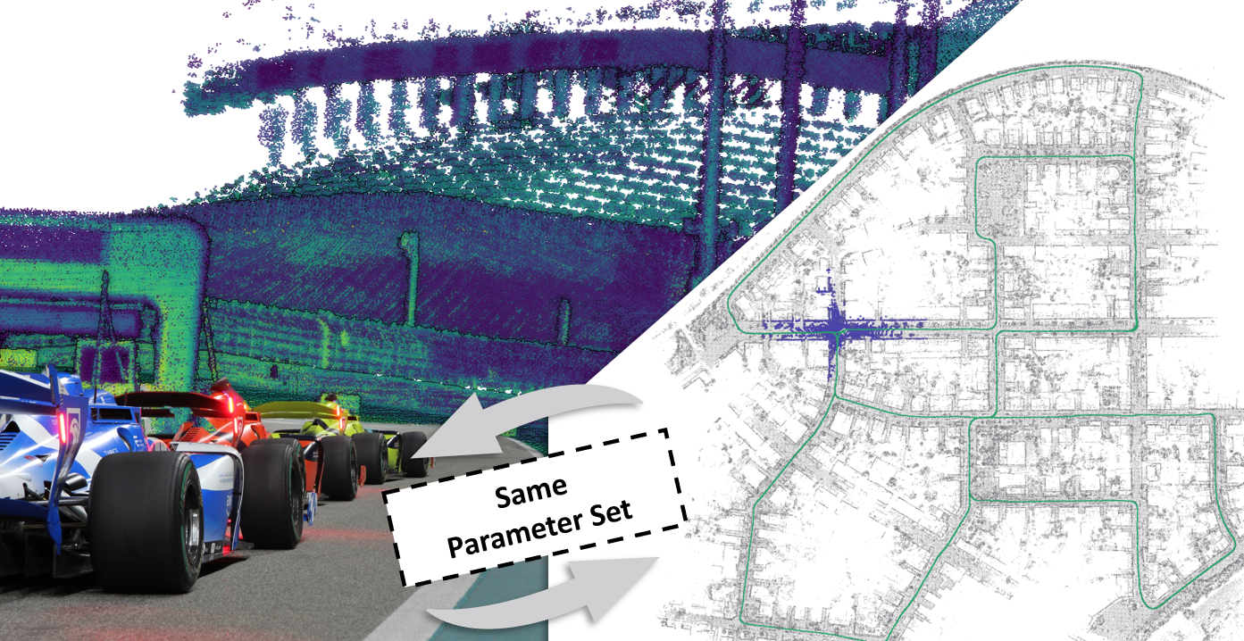
A year ago I wrote up FAST-LIO2 from scratch: one iterated Kalman filter, deskewed scans, point-to-plane residuals over an incremental k-d tree, 100 Hz on a laptop. That is the spine of modern LiDAR-inertial odometry (LIO), and it was built for drones and handheld scanners moving at human speeds. FAR-LIO, from TU Munich's Institute of Automotive Technology, asks a harder question: what breaks when the sensor is bolted to an autonomous race car doing 250 km/h, and how do you fix it without a different parameter file for every track?
Their answer is a different architecture. Not an iterated EKF registering raw points on a CPU k-d tree, but a CUDA scan pipeline — a voxel hashmap on the GPU, a sparsity-aware Generalized ICP, adaptive thresholding borrowed from KISS-ICP — feeding a small kinematic EKF that upsamples the IMU and compensates the pipeline's own latency. The headline, from the abstract: an average 6.9% lower positional error and 38.4% lower runtime than four baselines, on the race car's own compute, with a single parameter set across racetracks, highways and residential streets (reported). This is what each of those three contributions does, derived from the paper and checked against the shipped code — and where the numbers are more nuanced than the abstract line.
What LIO does, and why speed breaks it
LIO fuses two sensors that fail in opposite ways. A LiDAR gives tens to hundreds of thousands of accurate 3D points per sweep, but a sweep is slow (10–20 Hz here) and alone it is fragile to register. An IMU gives acceleration and angular velocity at hundreds of Hz — perfect for short-term motion — but it drifts. Register each scan against a running map to pin the pose, let the IMU carry you between scans, and each covers the other's weakness. I derived that loop in full in the FAST-LIO2 piece; here I take it as read.
At racing speed, three assumptions that are comfortable at walking pace stop holding. Slide the speed and watch why.
The whole scan is registered as if it were one rigid cloud. This much motion is baked into it — so every point must be deskewed first.
The IMU still samples motion finely at speed, so a linear velocity model across the sweep stays accurate. It is the only thing fast enough to undistort the scan.
The registered pose is already this far in the past when it reaches the filter. Delay compensation projects it forward to now.
- A sweep is not an instant. At 250 km/h the car covers 69.4 m/s. During one 10 Hz sweep
that is 6.94 m of travel (reasoned:
69.4 / 10); the scan the registration treats as a single rigid cloud was actually painted over seven metres of motion. Deskewing — projecting every point to the scan's final timestamp — stops being a nicety and becomes the difference between a map and a smear. - The IMU still resolves the motion. The race cars carry a Vectornav VN-310 at 800 Hz
(reported, Table I). Even at 250 km/h, two IMU samples are only 8.7 cm apart (reasoned:
69.4 / 800), so a simple linear velocity model across the sweep stays faithful. The IMU is the only thing fast enough to describe the within-sweep motion, which is exactly why the undistortion is driven from it. - Latency is a distance now. By the time a registered pose reaches the filter it is
already old. FAR-LIO's scan pipeline takes 19.23 ms on racing data (reported); that is
1.33 m of travel the EKF has to extrapolate away (reasoned:
69.4 x 0.01923). The paper shows in simulation that the error stays flat until the odometry lags by 60–100 ms, beyond which it diverges (reported, Fig. 5). At 250 km/h that threshold is 4–7 m — a wide margin only if your pipeline is fast and your filter closes the gap.
GICP correspondence is the fourth casualty, more subtly: at range, a single sweep is sparse, so the far-field points a racetrack needs for heading may have too few neighbours to estimate the surface covariance GICP wants. Hold that thought — it is the reason for one of the three contributions.
The architecture: a GPU scan pipeline and a CPU filter
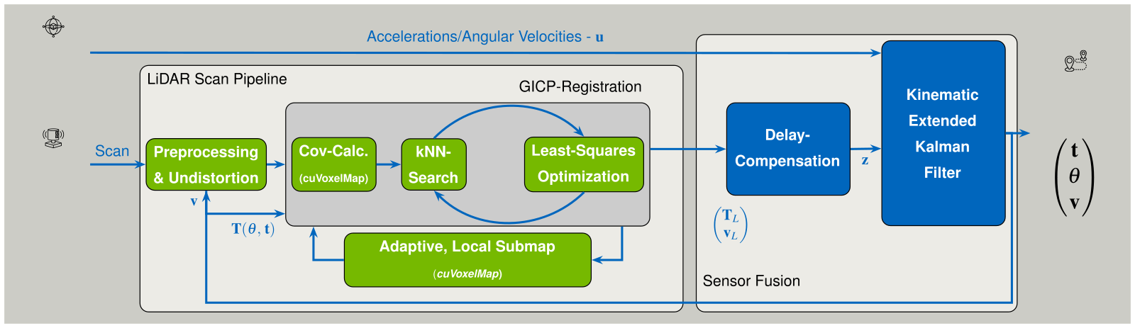
FAR-LIO splits cleanly in two. The LiDAR Scan Pipeline runs almost entirely on the GPU: it undistorts the incoming scan, computes point covariances, finds correspondences in a CUDA voxel map, and solves for the pose that registers the scan to a local submap. The Sensor Fusion backend runs on the CPU: a 100 Hz kinematic EKF that fuses that registered pose with the raw IMU, compensates its delay, and feeds its own estimate back as the next scan's initial guess. Click through the stages — the order is the order data flows.
what · Hash the query point to its voxel and scan the 27 voxels around it (3×3×3) for the nearest map point. The map is a CUDA hash table (cuco::static_map), iVox-style, v=4 m voxels holding up to N=40 points.
why · A flat hash table parallelises across thousands of GPU threads with no tree to descend or rebalance — the part a CPU k-d tree spends its scan budget on.
That split is the design. The expensive, embarrassingly parallel geometry — hashing points, searching neighbourhoods, building a least-squares system over thousands of correspondences — lives on the GPU, where FAR-LIO uses under 10% of an RTX A5000 on the open-source datasets and about 20% on the three-LiDAR racing setup (reported). The small, sequential, latency-critical state estimation stays on the CPU. All of it was evaluated on the dSpace AUTERA Autobox — an Intel Xeon D-2166NT (12 cores at 3 GHz) and an RTX A5000, the Indy Autonomous Challenge's official platform — with the algorithms pinned to four cores, the realistic budget for localization on a real car (reported). Now the three contributions.
1. A CUDA voxel hashmap with adaptive density
The map is where a CPU LIO spends its scan budget. FAST-LIO2's answer was the ikd-Tree — an
incremental k-d tree that inserts, deletes and rebalances in place. FAR-LIO throws the tree
out. Following the iVox paradigm (which the Faster-LIO authors argued beats tree structures
for this), it stores the map as a voxel hashmap on the GPU — cuVoxelMap, built on
NVIDIA's cuco::static_map. The key is a voxel's 3D integer index, hashed with Nießner et
al.'s spatial hash, collisions resolved by linear probing; each voxel holds up to a fixed
number of points. A k-nearest-neighbour query hashes the point to its voxel and scans the
27 voxels around it (a 3×3×3 block). No tree to descend, no rebalance — just a flat table
thousands of GPU threads hit at once.
The voxels are deliberately large: , up to regularly spaced points
each, which works out to a minimum spacing of about 65 cm between stored points (the first two
are reported in the paper; I confirmed voxel_size: 4.0 in the shipped config/far-lio.yml).
A big voxel captures enough local geometry to estimate a covariance, which GICP needs: for
each point, the covariance comes from its nearest neighbours and is regularised with
the Frobenius norm,
The config names the scheme outright — cov_regularization: "FROBENIUS", with "SVD" and
"MIN_EIGENVALUE" as the alternatives — so the paper's Eq. 1 and the shipped default line up
(measured, config/far-lio.yml).
The adaptive part — Adaptive Submap Density (ASMD) — is the generalization trick. Before
each update, FAR-LIO measures the average points-per-voxel in the current scan's near field and
caps the submap's density to match, with a linear decay over range and a floor of the
points a covariance needs. A dense racetrack scan and a sparse urban scan then produce submaps
of appropriate density without a hand-set voxel budget. Far voxels (beyond 1000 m of the
current pose) are dropped to bound the map — a limit the FAST-LIO2 authors used too, and one I
also found as max_distance: 1000.0 in the config (measured).
2. Sparsity-aware GICP with adaptive thresholding
Registration is GICP — align the scan to the submap by minimizing a Mahalanobis distance between corresponding point distributions, not raw points. Per correspondence of a source point to a reference point the residual is
and the pose solves a robust least-squares problem with a Cauchy kernel :
Two ideas on top make it work at speed, and both come straight from KISS-ICP. The first is
adaptive thresholding: rather than a fixed gate on correspondence distance, FAR-LIO tracks
the running deviation between where the IMU-driven initial guess said the scan would land and
where registration actually put it, and sets the rejection threshold from that. I read the
port in adaptive_threshold.hpp — it is KISS-ICP's Threshold.cpp almost line for line: the
model error is delta_trans + 2 * range * sin(theta / 2), accumulated into a sum of squares,
and the threshold is its RMS, capped at 10 m. When the car is being thrown around, the gate
widens to keep correspondences; when it is smooth, it tightens. One formula, no per-dataset
tuning.
The second is the sparsity-aware part (the SA in SA-GICP). When a source point sits somewhere too sparse to estimate a valid covariance — a far-field return on a wide track — the full GICP cost would drop it. FAR-LIO instead falls back to the degenerate case where is the identity and is zero, which is plain point-to-point ICP for that point. Those far points stay in the solve as point-to-point constraints instead of being discarded — and the ablation below shows that is a large part of what pulls down long-range drift.
The solve iterates until the update is tiny (,
which the config echoes as convergence_criterion: 5.0e-3) or it hits a time budget of twice
the LiDAR period — max_time: 200.0 ms, exactly 2 / 10 Hz (measured and reasoned). Better
to skip a frame than let one scan blow the latency budget the EKF depends on.
3. An EKF that compensates its own delay
The backend is small on purpose: a kinematic EKF at a fixed 100 Hz, a 9-dimensional state of position, orientation and velocity, taking IMU acceleration and angular velocity directly as control inputs,
Unlike FAST-LIO2, the IMU biases are not estimated online — they are calibrated once at standstill: fewer states to diverge under a race car's vibration, at the cost of assuming the biases hold for the run. The LiDAR pipeline supplies the measurement — position, orientation, a velocity differentiated from consecutive poses, and reference angles that stabilize roll and pitch to fight z-drift.
The interesting part is delay compensation. The registered pose is ~19 ms old when it arrives; applying it as if it were current would yank the estimate backwards. FAR-LIO instead extrapolates it to the present using the filter's own state history,
where is the measurement's true timestep, is now, and is the measurement model. The same mechanism lets FAR-LIO upsample one LiDAR pose into several EKF corrections, spreading its influence over multiple 100 Hz cycles so the output is smooth enough for a controller to drive on. This is the piece that turns a fast-but-bursty scan pipeline into a steady, low-latency pose stream.
Checking the claims
The headline racing comparison is the point of the paper, so it is the number to check.
On the Abu Dhabi (Yas Marina) and Monza sequences, absolute positional error (APE, RMSE in
metres) and relative positional error (RPE, % per 100 m), computed with evo, best in bold
and "x" meaning no valid result (all reported, Table II):
| Sequence | FAST-LIO2 | D-LIO | KISS-ICP | Faster-LIO | FAR-LIO |
|---|---|---|---|---|---|
| yas_10 (APE) | 37.24 | 19.70 | x | 36.00 | 15.68 |
| yas_20 (APE) | 50.13 | 45.23 | x | 55.71 | 25.62 |
| mon_20 (APE) | 262.16 | x | x | 475.28 | 297.39 |
| yas_10 (RPE) | 2.14 | 4.34 | x | 3.30 | 1.67 |
| yas_20 (RPE) | 2.08 | 3.31 | x | 3.07 | 1.84 |
| mon_20 (RPE) | 4.44 | x | x | 7.06 | 2.74 |
On the two Yas Marina sequences FAR-LIO wins outright: 15.68 m APE on yas_10 against the
next-best 19.70 (D-LIO), a 20.4% reduction (reasoned: (19.70 - 15.68) / 19.70), and
25.62 against 45.23 on yas_20, a 43.4% reduction (reasoned). KISS-ICP, the pure-LiDAR
baseline, produces no valid result on any racing sequence.
Monza (mon_20) is where honesty matters: FAR-LIO's APE of 297.39 m is worse than FAST-LIO2's 262.16 m (reported). FAR-LIO does not sweep every cell. What it does do is post the best RPE on all three racing sequences — 2.74 on mon_20 against 4.44 and 7.06 — and it is one of only three methods to return a valid result there at all. The 6.9% headline is a combined average of APE and RPE across all datasets (reported), not a clean APE victory; read as "best local consistency everywhere, best global accuracy almost everywhere, and the only method that finishes every sequence," which the paper states plainly: every baseline fails at least one sequence, FAR-LIO finishes all of them.
The ablation earns the three pieces
The component study on the Yas sequences is the cleanest evidence that each contribution pays for itself — and that they do not all push the same metric (all reported, Table III, yas_10):
| Configuration | APE (m) | RPE (%) |
|---|---|---|
| Constant-velocity baseline (no EKF) | 66.32 | 6.94 |
| + EKF | 45.34 | 1.94 |
| + delay compensation | 21.46 | 1.97 |
| + motion undistortion | 28.09 | 1.66 |
| + sparsity-aware GICP | 16.11 | 1.66 |
| + adaptive submap density (full) | 15.68 | 1.67 |
From 66.32 m to 15.68 m is a 76.4% drop in APE (reasoned), and the RPE collapses from 6.94 to 1.67 the moment the EKF replaces the constant-velocity assumption. But look at the motion undistortion row: it raises APE from 21.46 to 28.09 while cutting RPE from 1.97 to 1.66. Deskewing buys local consistency (RPE) at a temporary cost in global accuracy (APE) — and it is the sparsity-aware GICP and adaptive density that then pull APE down hard, 28.09 to 16.11 to 15.68. The pieces are complementary, not individually monotonic, which is exactly the kind of detail an abstract average hides.
Runtime: the 38.4%
FAR-LIO's total callback time is 19.23 ms on the three-LiDAR racing data (about 200,000 points per concatenated scan) and 9.59 ms on the single-LiDAR open-source datasets (reported). Faster-LIO, the only baseline with comparable speed, runs 50.01 ms and 18.55 ms; FAST-LIO2, DLIO and KISS-ICP cannot keep up with the sensor rate or diverge on the racing data (reported). The abstract's 38.4% lower runtime is an average over the baselines and datasets — I could not reproduce that exact figure from the two callback numbers alone (FAR-LIO is 48–62% faster than Faster-LIO on each set, a larger margin), so 38.4% is the conservative cross-dataset average, not the race-car number. The practical point stands: at 19.23 ms, on 20% of one GPU, FAR-LIO sits far below both the sensor period and the 60–100 ms divergence cliff.
A sidebar: how you'd test an LIO system in sim
You do not get a race car to debug on. Before FAR-LIO ever sees a track, you shake out an LIO stack in simulation — and the hard part of a faithful LiDAR sim is reproducing the scan pattern, because that is what the deskew and the correspondence search assume. A spinning Velodyne is easy; a Livox-style solid-state sensor with a non-repetitive pattern is not.
ashduwihch/mid360_gazebo_harmonic
(MIT) is a neat example. Gazebo Classic reached end-of-life in January 2026 and the old
livox_laser_simulation plugin does not run on the current engine, so this project ports a
Livox Mid-360 simulator to Ubuntu 22.04, ROS 2 Humble and Gazebo Harmonic. It replays a
recorded Mid-360 scan order for the real non-repetitive pattern, emits 200,000 points/s at
10 Hz (20,000 rays per frame), and preserves line, offset_time, tag and reflectivity
— crucially offset_time, the per-point timestamp a deskew needs. It publishes
sensor_msgs/PointCloud2, Livox's livox_ros_driver2/CustomMsg and sensor_msgs/Imu, so it
drops straight into a FAST-LIO2 ROS 2 graph, ray-casting against Gazebo collision geometry
with Embree via a vendored copy of rmagine (BSD-3, Alexander Mock).
The Mid-360 is a different sensor than the race cars' Seyond Falcon and Luminar Iris, so this is not a FAR-LIO rig as-is. The point is the methodology: a simulator that emits a physically faithful non-repetitive scan, with per-point timestamps, is how you validate the undistortion and registration of any Livox-fed LIO before you trust it on hardware.
- license
- Apache-2.0
- branch
- main
- tests
- 24 files
- source
- 939.8 kB
- commit date
- 2026-09-22
by size of tracked source at this commit, file counts in brackets; docs, data and vendored trees excluded
local clone, 2026-10-02 at ef20510 — branch, commit, commitDate, fileCount, hasTests, languages, license, licenseFile, shallow, testFileCount
shallow clone: counts describe the pinned tree, not the history
- license
- MIT
- branch
- main
- tests
- none found
- source
- 491.2 kB
- commit date
- 2026-09-29
by size of tracked source at this commit, file counts in brackets; docs, data and vendored trees excluded
local clone, 2026-10-02 at b95e11b — branch, commit, commitDate, fileCount, hasTests, languages, license, licenseFile, shallow
shallow clone: counts describe the pinned tree, not the history
Honest notes
- I did not run it. There is no race car and no A5000 in my sandbox, and the system is a ROS 2 Jazzy / CUDA / C++20 stack meant for one. Every number here is checked against the paper and the Apache-2.0 code and config, not re-measured. The APE table, the ablation, the 6.9% and the 38.4% are the authors' reported figures; my own numbers (the per-sweep distances, the 20.4%/43.4%/76.4% reductions, the 200 ms budget arithmetic) are labelled reasoned and derived from theirs.
- The biases are a bet. Calibrating IMU bias once at standstill trades online adaptability for fewer states to diverge. On a short, violent race run that is clearly the right call; on a long run with thermal drift it is a known limitation the paper accepts.
- It is odometry. RPE — local consistency — is FAR-LIO's strongest axis, which is what a closed-loop controller cares about. Global APE on very long sequences is still large for everyone (MulRan Sejong is in the thousands of metres across all methods); FAR-LIO has no loop closure, by design, and mon_20 is best read as best-RPE plus finishing-every-sequence, not a clean APE win.
The thing I would take away: FAR-LIO is a rethink of where LIO should compute. FAST-LIO2 put a clever incremental tree and a reformulated gain on a CPU; FAR-LIO moves the whole geometry — a hash-table map, a sparsity-aware GICP, adaptive thresholds — onto the GPU, keeps a tiny delay-compensating EKF on the CPU, and spends the latency it saves on a margin against divergence. That it does so with one parameter set from a residential street to a 250 km/h straight is what makes it worth reading.
Built on FAR-LIO: Enabling High-Speed Autonomy through Fast, Accurate, and Robust
LiDAR-Inertial Odometry (Leitenstern, Weinmann, Haft,
Lasser, Kulmer, Lienkamp; TU Munich, IROS 2026) and the Apache-2.0
TUMFTM/FAR-LIO source and config. GICP and adaptive
thresholding follow KISS-ICP (Vizzo et al.); the iVox map
paradigm follows Faster-LIO (Bai et al., IEEE RA-L 2022). Related here:
FAST-LIO2 from scratch,
SurfSLAM, GTSAM 4.3, and
Depth Anything 3 in ROS 2.