Gaussian-splat capture in practice: from a 360 camera to a scene on a map

mdjsonmcpcopy↗ai

2026-10-06 · 21 min · 3d · gaussian-splatting · slam · webgpu · point-cloud

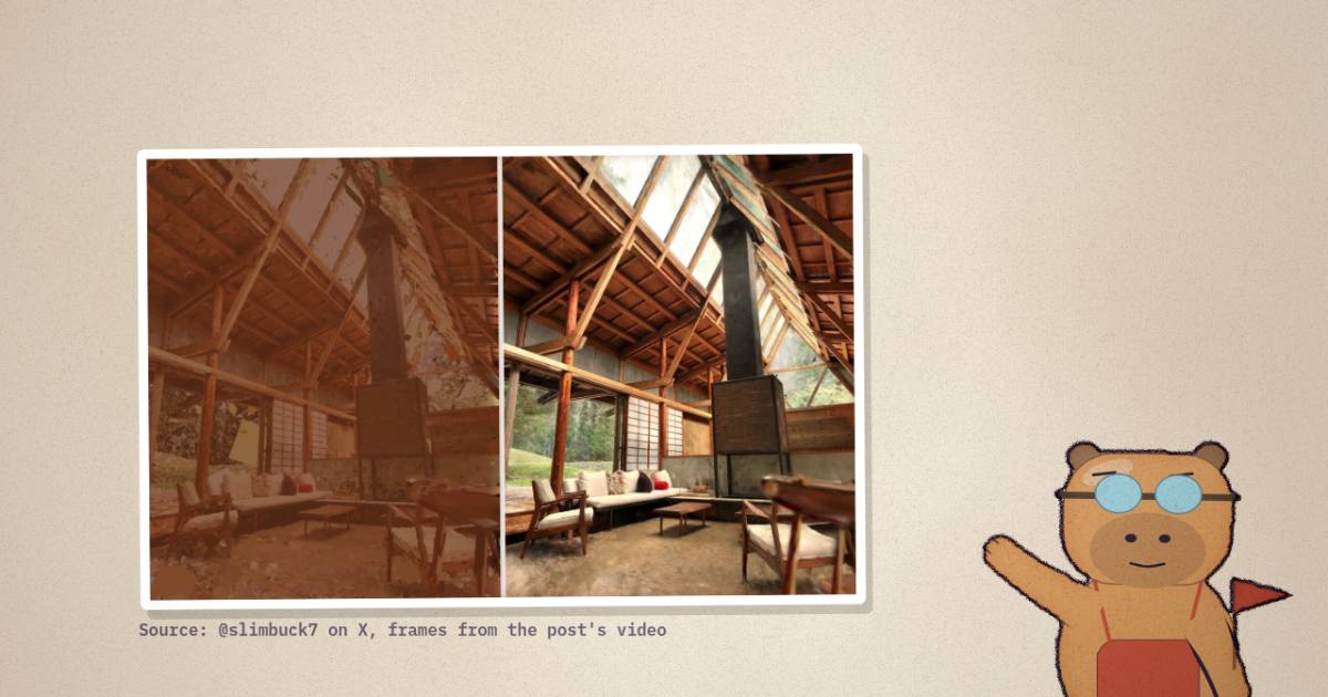
A year ago a good Gaussian-splat scene meant a mirrorless camera, careful stills, COLMAP overnight and a research trainer. This fortnight's posts describe something else. A dam in Japan flown once with a 360 drone. A two-kilometre shrine approach walked with a 360 camera on a stick. A phone streaming GPS to the camera so the finished splat lands on a map at the right size. A browser drawing three million splats on a three-year-old phone without sorting them.

None of these is a paper. They are pipelines. I read the posts, their threads and replies, the pipeline guide one of them maintains, and the source of the tools they name: LichtFeld Studio, Spirula Studio, metal-gauss and the PlayCanvas engine. Every number below is labelled: reported is the poster's or the project's figure, measured is something I read off a file or a frame, and reasoned is my arithmetic on the other two.

The splat format itself, and why a 1.18 GB PLY becomes a 65 MB SOG, is in SOG: a Gaussian splat scene as spatially-ordered WebP images. Spirula Studio's internals are in Spirula Studio deleted its dependencies instead of wrapping them. This piece is the part before and after: capture, alignment, scale, training budget and rendering.

The pipeline, stage by stage

Every source here runs the same seven stages: capture with a 360 camera, flown or walked; projection, the sphere stored as two fisheye circles, one equirectangular panorama (ERP) or six cube faces; frames and masks, the sharpest frame per interval with the operator, the drone's parts and the stitch seam masked out; structure from motion, every camera pose plus a sparse cloud; scale, because images fix a scene only up to a similarity transform; training; and delivery, compression or tiling plus a renderer. They differ in what they pick at each one.

A dam from one drone flight

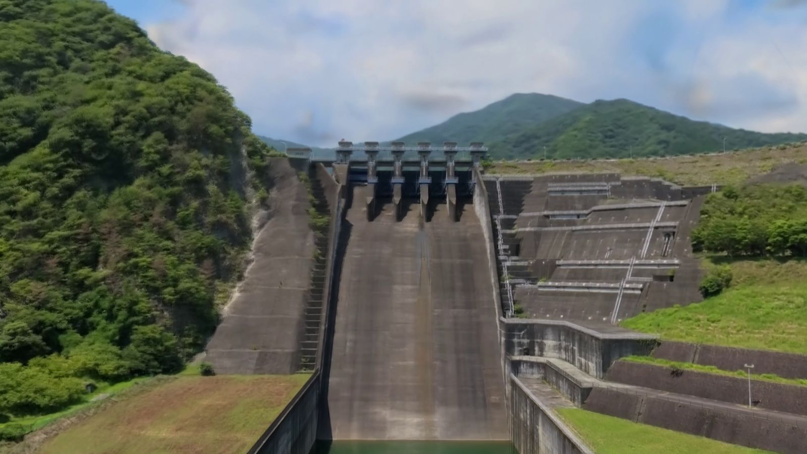
@kotohibi_3d's Miho dam is the most fully documented capture in the set. The post lists the steps; the replies add the training cost. All reported:

• DJI Avata 360, one flight, 14:34 of 8K D-Log M video.
• 875 masked frames, extracted with the author's own tools.
• Spherical SfM in Metashape Standard, with the masks.
• Cubemap conversion and "parallax-based reduction".
• LichtFeld Studio: 15M splats, SH2, strategy MRNF, PPISP on.
• AprilTag real-scale estimation, in a follow-up post.
• Training took "around 14 hours with RTX 4090 24GB", 481,300 iterations. Asked why SH2 and not SH3: "VRAM limitation".

expand

The author also maintains a CC BY 4.0 pipeline guide, the best description of a 360-to-splat workflow I have found. Frames come from a tool that keeps the sharpest frame per chunk. Masks come from YOLO classes or a SAM 3 text prompt, plus a seam mask for the stitch line between the two fisheye lenses. That seam mask only works if in-camera horizon levelling is off, because levelling moves the seam.

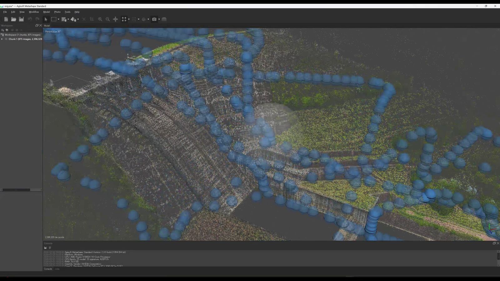
In Metashape, the camera type is set to Spherical, masks are applied to key points, and then the tie points are cleaned in three passes: reprojection error, reconstruction uncertainty and projection accuracy, about 5% each, re-optimising the cameras after each pass, twice round. It is classic photogrammetry hygiene, and the guide calls it "a very important step for high-detail 3DGS".

expand

Why equirectangular for SfM, and cube faces for training

A dual-fisheye 360 camera is two cameras about 3 cm apart, back to back. If you hand an SfM tool the two fisheye streams, it sees two cameras per instant that share almost no features with each other, so it has to discover that they are a rigid rig. Spirula's own notes say this plainly, about a GoPro MAX unwrapped into ten views per frame: without a rig constraint, a 78 s handheld walk reconstructed as 645 of 930 images over 3 components (reported, docs/notes/sfm-rig-constraints.md). The same note says why an ERP aligns more easily: "it is one camera, so the connection between what the six directions see is not something the mapper has to discover."

So the 360 practitioners solve poses on the ERP, with a spherical camera model. Then they cut each panorama into cube faces for training, because most trainers rasterise pinhole cameras, and an ERP's poles are smeared across a whole image row. The resolution survives the cut. An 8K ERP spreads 7,680 px over 360°, about 21.3 px per degree; the guide's recommended crop of 1,920 px for a 90° cube face is the same 21.3 px per degree (reasoned). The guide's converter also adds a yaw offset of 5–30° per frame, so the face boundaries do not fall on the same bearings in every frame.

Parallax-based reduction

Six faces per frame is a lot of near-duplicate images when the camera crawls. The guide's converter drops whole source frames whose neighbours already cover them. The example in the guide keeps 237 of 251 source frames and removes 14 (5.6%), taking 1,506 cube faces to 1,422, under thresholds of a 3.0 maximum camera distance, 4.0° maximum foreground parallax and at least 100 shared visible points (reported, read off the screenshot below).

expand

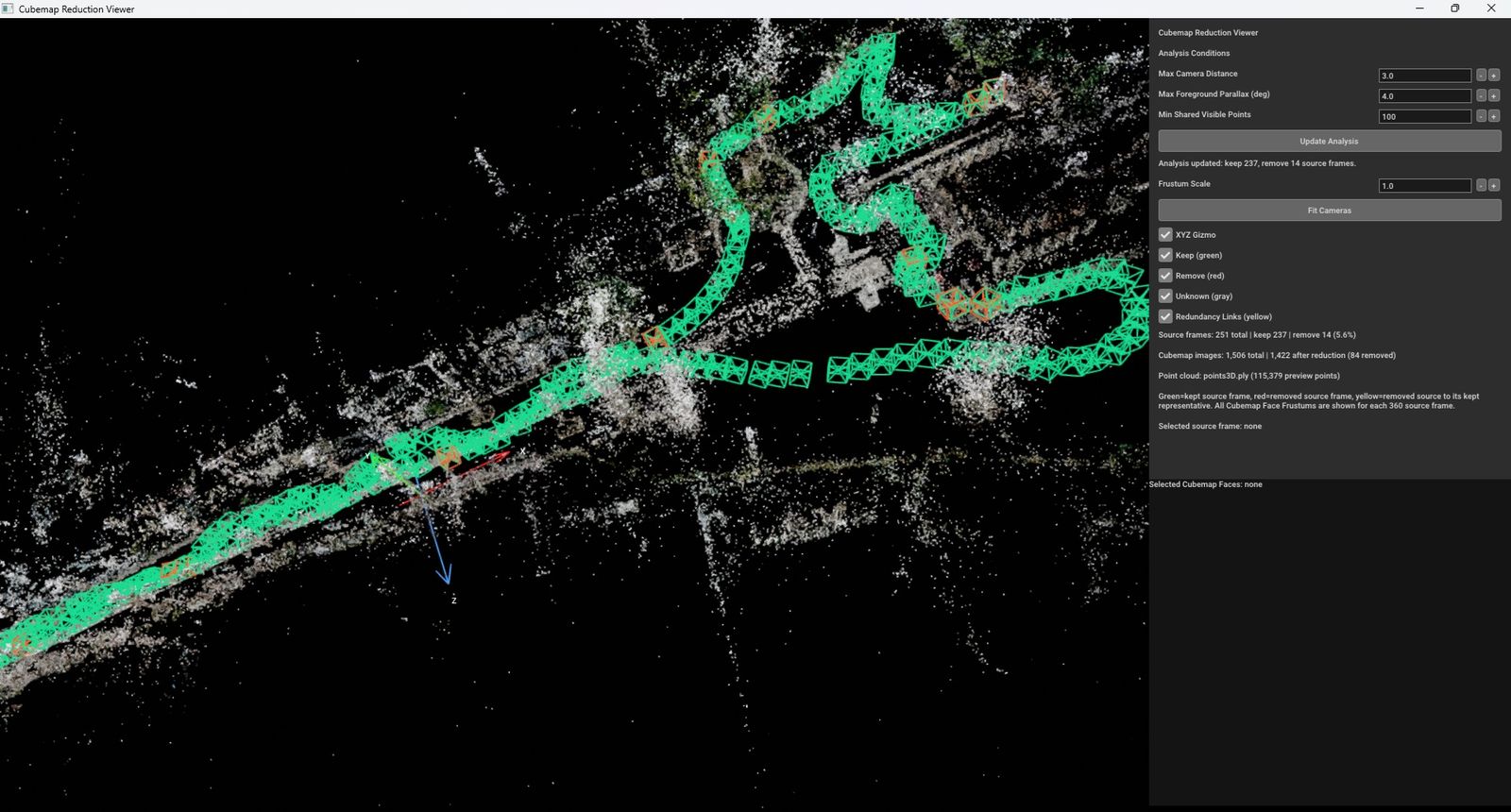
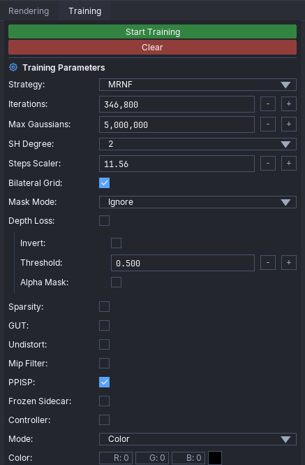
For the dam, I can back out roughly how many images went into training. LichtFeld Studio's GUI auto-scales the step count by image count: autoScaleSteps sets the scaler to image_count / 300 above 300 images (src/visualizer/core/parameter_manager.cpp), on a base of 30,000 iterations. The guide's own screenshot shows 346,800 iterations with a steps scaler of 11.56, which is exactly 30,000 × 11.56. So 481,300 iterations means about 4,813 training images. Six faces from each of 875 frames is 5,250, so the reduction removed roughly 437 faces, about 8% (reasoned, assuming the default auto-scale was left on). And 481,300 iterations in about 14 hours is about 9.5 iterations a second on the 4090 (reasoned).

Scale from AprilTags

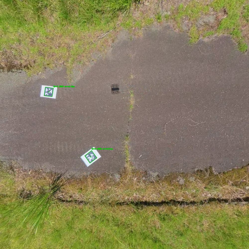
SfM recovers a scene up to an unknown scale. The dam's follow-up post shows the fix: printed AprilTags on the ground, detected in a cube face, each marked USED with a corner reprojection error of about 0.2 px (measured, read off the image). With the tag's printed size known and its corners triangulated from several views, the ratio of the two lengths is the scale. It is the cheapest metric reference there is: a sheet of paper.

expand

What MRNF and PPISP are

The guide recommends LichtFeld Studio's MRNF strategy "at the time this article was written" and says PPISP often replaces the bilateral grid. Neither acronym is expanded anywhere I could find in the repository. The UI calls it the "Default 3DGS strategy with MRNF refinement". The code is readable (src/training/strategies/mrnf.cpp). Each refine window it soft-prunes splats with near-zero opacity, a degenerate rotation, a collapsed scale or an absurd extent, and parks their rows in a free list. Then it grows: a fraction of the candidates, grow_fraction 0.07 by default, is picked by Gumbel top-k sampling weighted by an SSIM-based error map and an edge score, and split into children that reuse the freed rows first. On top sit opacity decay and noise injection on the means, ideas recognisable from MCMC-style 3DGS. The default max_cap is 5,000,000 splats; the dam raised it to 15M.

PPISP is easier: it is NVIDIA's Physically-Plausible Image Signal Processing, vendored under Apache-2.0. It learns a per-camera ISP: exposure in EV stops, vignetting, a colour correction over four chromaticity control points, and a camera response curve with toe and shoulder (src/training/components/ppisp.hpp). It keeps exposure and white-balance drift between frames out of the splats' colours, which matters over a 14-minute flight.

expand

Why SH2: the splat budget

The "VRAM limitation" answer is checkable arithmetic. A splat's view-dependent colour is a spherical-harmonic expansion with $(d+1)^2$ coefficients per colour channel: 1, 4, 9 and 16 for degrees 0 to 3. A standard 3DGS PLY stores, per splat, position (3), normals (3), the DC colour (3), the rest of the SH ($3((d+1)^2-1)$), opacity (1), scale (3) and a quaternion (4), all float32. That is 68, 104, 164 and 248 bytes per splat; the 248 B at SH3 matches what the SOG article measured on a real file.

At 15M splats, an SH2 PLY is about 2.46 GB and an SH3 one about 3.72 GB (reasoned). Training is worse. The trainable parameters (no normals) are 38 floats a splat at SH2 and 59 at SH3, and a naive fp32 trainer holds each one four times over: value, gradient and the two Adam moments. That is 9.12 GB for 15M splats at SH2 and 14.16 GB at SH3, before a single image buffer or the rasteriser's scratch (reasoned). LichtFeld Studio quantises the higher-order SH by default (LFS_SH_VALUE_QUANT), so its real figure is lower; but with thousands of 1,920 px images and the densification bookkeeping also resident on a 24 GB card, dropping a degree is the obvious lever. The second panel is the rendering budget, covered at the end.

A shrine approach on foot, and why the fisheye file failed

DuckbillStudio walked the approach to Togakushi Shrine's Okusha with a DJI Osmo 360: 2 km in 40 minutes, the famous cedar avenue beyond the red thatched Zuishin-mon gate. The splat was built in Spirula Studio from 360 video converted in DJI Studio. The thread adds (all reported): the 10 clips were merged into 3 ERP videos in DJI Studio with a LUT applied; just under 400 extra stills were shot around the gate; and with the dual-fisheye .osv files "parts that would not connect always appeared, whatever extraction interval or alignment method I used, but with ERP every frame connected" (my translation). Asked about training, the author says it was about 5,000 images at 8K equirectangular, processed all at once with no block-based training, with "no problem at all" on an RTX 4090.

expand

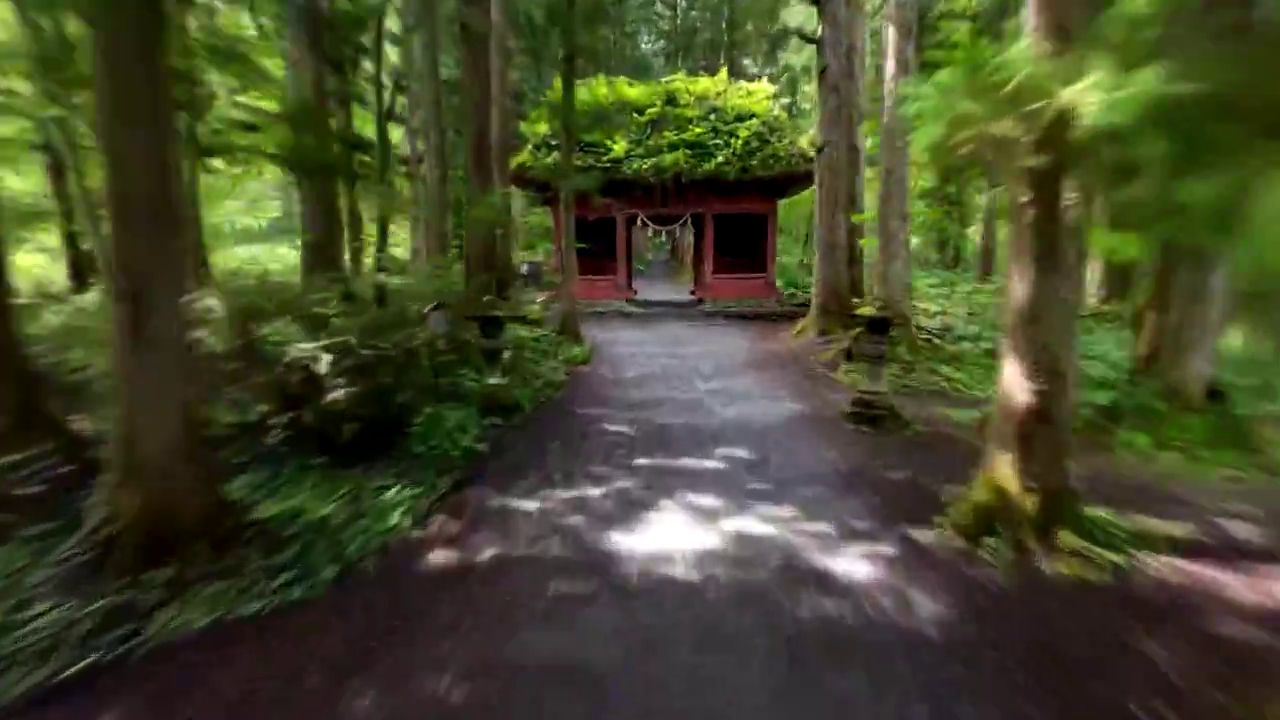
This is the rig problem from above, met in the field. The ERP turns each instant into one camera. The .osv makes the solver find the second lens on its own, frame after frame, through a forest where neighbouring frames share mostly foliage. The SfM result in the thread is a single unbroken strand two kilometres long, 2,777,150 points (measured, the counter in the screenshot).

expand

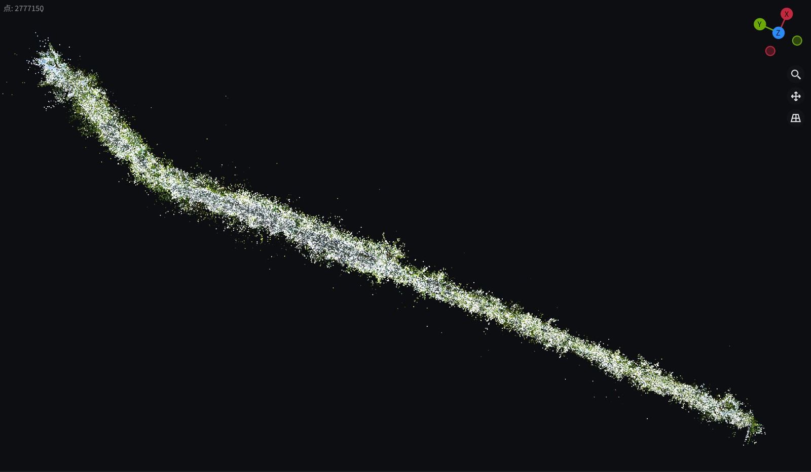
Two kilometres in 40 minutes is about 0.83 m/s (reasoned): a slow walk, more overlap per metre, less blur. The author's shorter follow-up is the same split for ordinary photos: Spirula Studio for SfM, LichtFeld Studio for training, which "might be the better combination" for a normal photo set. LichtFeld's maintainer replied that SfM "is coming soon to lfs".

Putting the splat on a map

DuckbillStudio's third post closes the loop from capture to a map. The steps (reported):

1. An Android app reads the phone's GPS and sends it, with shutter control, over Bluetooth Low Energy to one or more Osmo 360s.
2. Each camera writes the position into its video.
3. Spirula Studio runs SfM with a weak position constraint, giving a correctly scaled splat.
4. Optional cleanup in SuperSplat.
5. Conversion to geo-referenced 3D Tiles, including a rescale.
6. Display in a map viewer.

The quoted post says the camera-to-scaled-splat half took a day to build.

expand

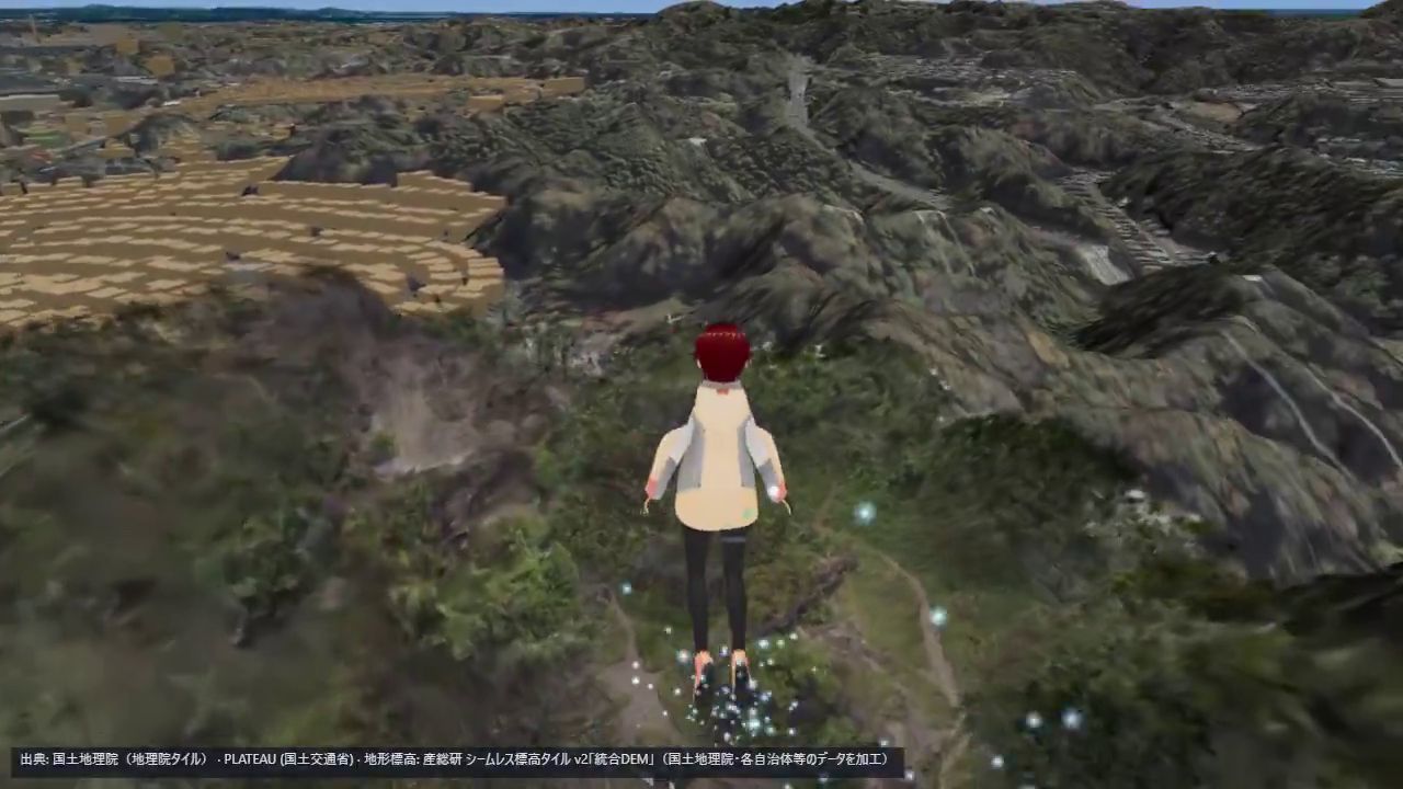
"Weak" is the important word, and Spirula's notes say why. Consumer GPS is good to a few metres; their GoPro MAX example reports a DOP around 2, which "with a typical 3-5 m range error means 6-10 m horizontal" (reported, docs/notes/imu-gps-for-sfm.md). Worse, the error is correlated over minutes. Spirula's implementation therefore adds GPS as a per-frame position factor with the receiver's sigma and a Huber loss inside bundle adjustment, so that "one wrong prior -- a synchronisation glitch, a wild GPS fix -- bends nothing" (docs/notes/sensor-priors.md). Vision decides local geometry; GPS decides scale, long-range drift and placement. For scale alone, the note reports 0.2 percent from GPS over a 100 m walk.

There is a hardware detail here too. Spirula's survey of the .OSV format found the Osmo 360 files they had carry a 1 kHz fused attitude quaternion and no GPS, although their reader knows where the Osmo's GPS fields sit. The same note found the Insta360 X5's GPS log "is the phone's position pushed over Bluetooth". So a 360 camera's GPS is usually a phone's GPS, and it is only there if a phone was connected while recording. DuckbillStudio's Android app makes that connection deliberately, for several cameras at once, and adds the shutter. I cannot see the app; this is my reading of how step 2 squares with the file format.

LichtFeld Studio on Metal

The training half of the dam pipeline was CUDA-only until recently. @janusch_patas (MrNeRF), LichtFeld's maintainer, posted it running on a Metal backend with split viewports: splats, rings and the point cloud side by side while training continues.

expand

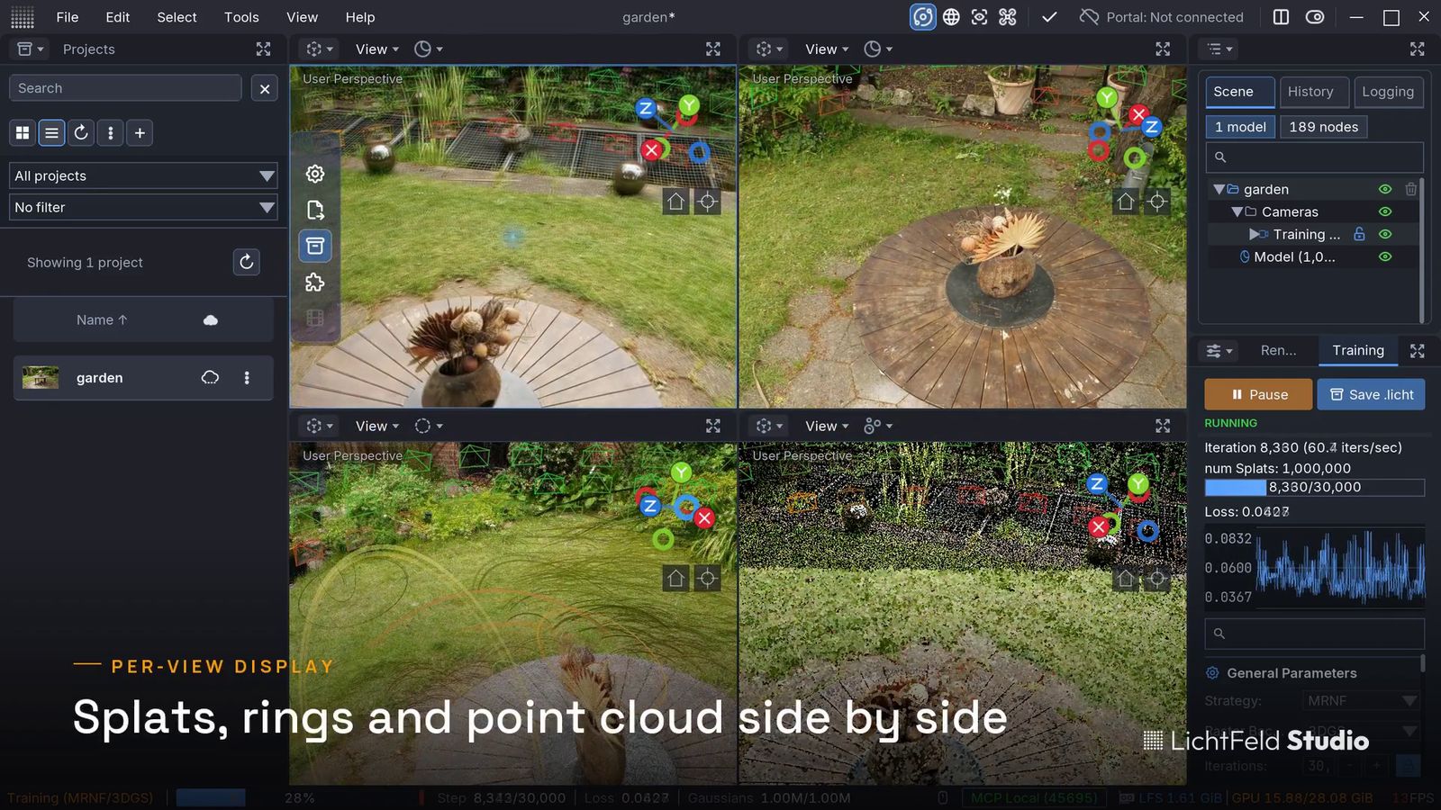
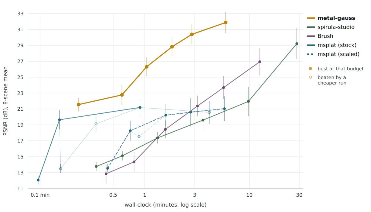
Asked about speed, he answered "Slower :D … It is certainly slower than 2x on my M5", with measurements promised later; a test release was promised for "some time next week" (reported). In the replies, Nando Metzger linked metal-gauss, and janusch confirmed: "I used the rasterizer as base". So the link is relevant: metal-gauss is a 3DGS trainer on Apple Silicon with Metal kernels compiled at runtime, no CUDA, no Xcode. Its tile binning uses an exact ellipse-tile test that drops 38.7% of tile-Gaussian pairs with a bit-identical image, and SSIM and Adam run entirely in Metal (docs/ARCHITECTURE.md).

Its README benchmarks quality per minute on an Apple M5 with 24 GB, across the 8 NeRF-synthetic scenes (reported). Given 30 s, metal-gauss reaches 21.6 dB mean PSNR against Spirula Studio's 13.8; at 6 min, 31.3 against 19.6; at 30 min, 31.9 against 28.5. Those are small object scenes on a laptop chip, not a dam, so read them as a statement about the Metal kernels, not about which trainer to use for a 15M-splat capture.

expand

Rendering without sorting

The last stage is drawing the thing. Standard 3DGS composites translucent splats front to back, so every frame needs every visible splat sorted by depth from the current camera. Move the camera and the order changes; re-sort. That sort is memory-bandwidth work over millions of keys every frame, which is what a phone lacks.

Donovan Hutchence (@slimbuck7), who works on PlayCanvas and SuperSplat, posted the alternative: "7.5 ms a frame on a Pixel 7 Pro in Chrome/WebGPU, where sorting takes 19.5" (reported). At 60 Hz the frame budget is 16.7 ms, so the sort alone overruns it, and the stochastic frame fits with room to spare (reasoned). The catch is in the same post: "The flickery blobs are a per-frame thing; over time they resolve to the correct image. Too flickery to ship as-is", with a better-resolving, slower version already in hand.

expand

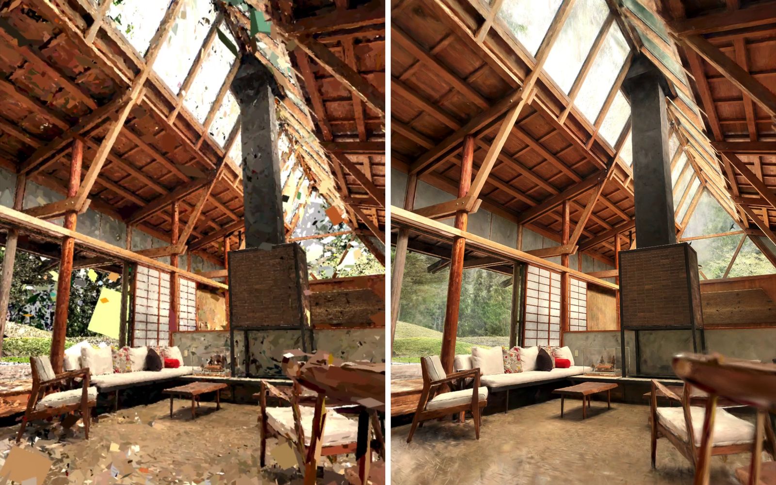
Why it works is one line of probability. Sorted alpha blending gives splat $i$ the weight $\alpha_i \prod_{j \text{ in front}} (1-\alpha_j)$. Now draw every splat opaque, with depth testing, but let each fragment survive only with probability $\alpha_i$, by comparing $\alpha_i$ against a noise value. A fragment is the visible one exactly when it survives and every fragment in front of it does not, which happens with probability $\alpha_i \prod_{j} (1-\alpha_j)$: the same weight. The depth buffer does the ordering for free, in any draw order. One frame is a noisy sample of the right answer; averaging frames, with temporal anti-aliasing, converges to it.

That is what PlayCanvas's engine ships today as GSplatParams#stochastic: on the WebGPU GPU-sort renderer, "Splats are drawn without sorting, using dithered coverage, opaque blending and depth writes", with blue noise as the default dither because it "looks best under temporal anti-aliasing"; picking still uses the sorted path (src/scene/gsplat-unified/gsplat-params.js, read at 9f0f464). With the flag on, the projector writes stable splat IDs instead of sort keys and the radix sort is skipped outright. Off, the key width is round(log2(N/4)) clamped to 10–20 bits, which for 3,289,356 splats is 20 bits, rounded up to the sorter's 8-bit digit for the OneSweep backend (reasoned from gsplat-hybrid-renderer.js).

The demo in the post goes further than the shipped flag. In the replies, slimbuck explains the visibly spinning billboards: they rotate "so that once you average the result over many frames, it converges to the usual blended version", spinning in 2D "to get the gaussian falloff over time", and he confirms this needs no fragment shader and is "novel". I did not find that variant in the engine's main branch; what is there is the dithered one.

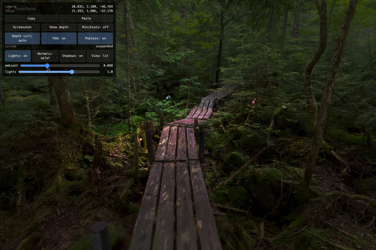
A depth buffer is the other dividend. Opaque surviving fragments mean the splats have a depth, which is what a shadow map or a lit pass needs. slimbuck's earlier post shows dynamic point lights with shadows on a DuckbillStudio forest scene, attributed to the same stochastic approach.

expand

Photos back where they were taken

The fifth post points the pipeline the other way. Instead of building a 3D scene from your own images, Shadnam Khan of MultiSet places other people's photos of Westminster into an existing 3D model: "each one dropped back at the exact spot and angle it was taken from. We didn't scan anything. Testing on Google's 3D Tiles." In a reply he says the photos came from Google image search.

That is visual positioning (VPS), not reconstruction. For each query photo you find local features, match them to features attached to the 3D map, which turns them into 2D-to-3D correspondences, and solve the camera's 6-DoF pose with PnP inside RANSAC. The map does not have to be yours; here it is Google's photogrammetric tiles. MultiSet's site claims "≤5 cm accuracy" and localisation against maps built from LiDAR, meshes, Gaussian splats or 360 video (reported, product page; not tested in the post). Repliers pointed out that Photosynth did a version of this years ago; what is new is that the map already exists, at city scale.

expand

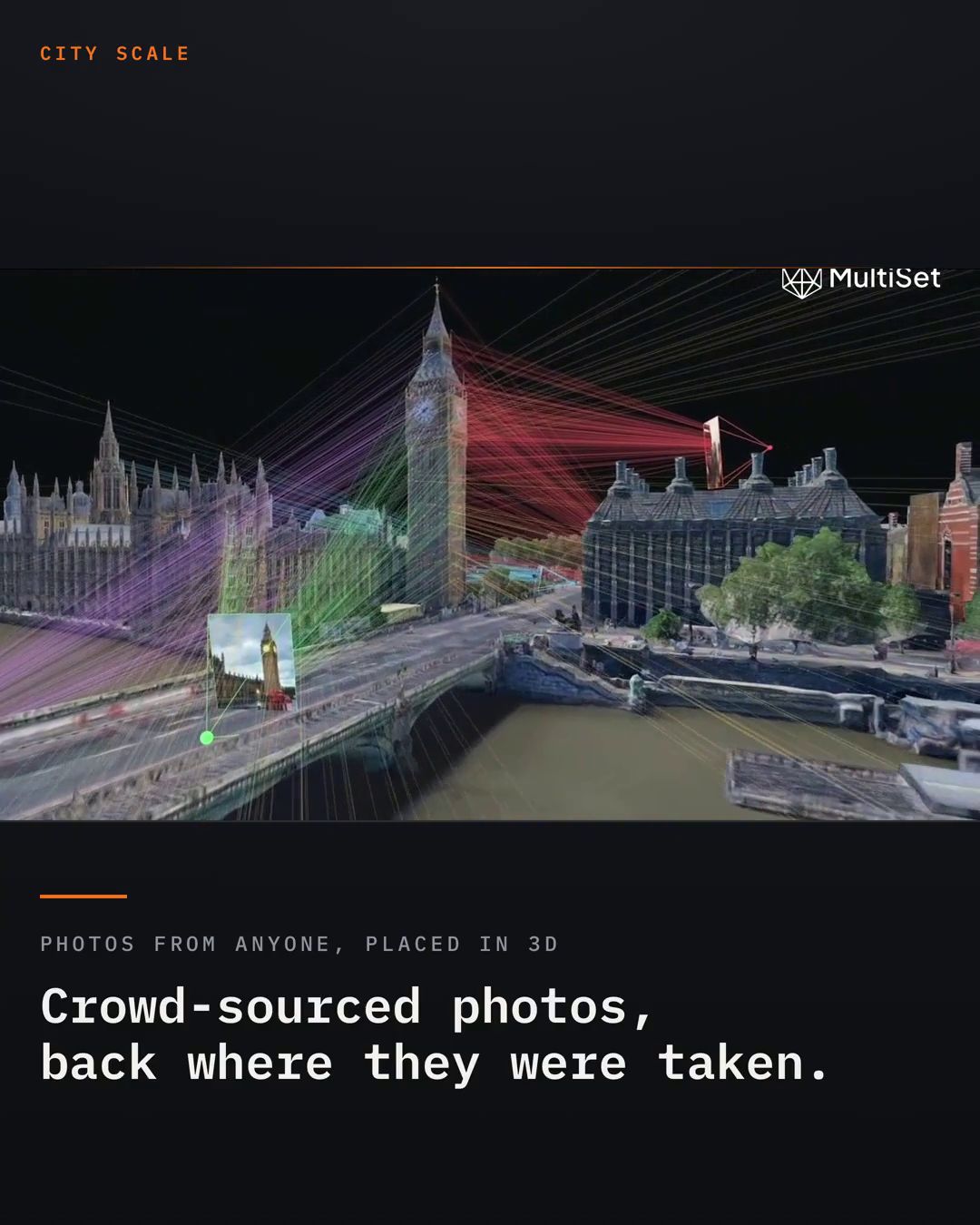
For a splat pipeline, this is the same scale-and-place problem as the GPS stage, solved with pixels instead of a receiver: localise a few of your frames against a geo-referenced map and you have scale and placement without AprilTags or a phone.

What I would take from this

• Solve poses on the ERP, train on cube faces. The dual-fisheye route breaks on long captures because the solver has to discover the rig; a 1,920 px face at 90° keeps an 8K ERP's resolution.
• Give it scale on day one. A printed AprilTag, or a phone's GPS as a weak prior, and the splat drops into 3D Tiles at the right size.
• SH degree is the VRAM dial; on phones, the sort is the frame-time dial. SH2 instead of SH3 cuts the PLY from 248 to 164 bytes a splat; stochastic transparency removes the sort at the cost of noise that only time averaging hides.

What I could not check: none of the capture numbers can be re-run without the footage, so they stay reported; MRNF's name is not expanded anywhere I could find; janusch's Metal speed ratio is a reply, not a benchmark; and slimbuck's 7.5 and 19.5 ms are his phone measurements, while the HUD in his recording shows GPU times of 4.3–5.0 ms on a device the post does not identify.

Related: the pose problem these tools solve offline is the one streaming reconstruction from unposed video tries to solve online; the newest feed-forward methods are in the first and second 3D roundups; and once a splat exists, Carveout labels its objects with SAM 3.