2026-10-16 · 19 min · 3d · gaussian-splatting · lidar · slam · point-cloud · robotics
A 1:46 narrated explainer, drawn in code. Every number and picture in it is this article's own; the sources are below.
› transcript
Hi, I'm Parallax! Hesai makes lidar for cars. Now it sells a handheld that turns a room into a Gaussian splat. Photos alone cannot tell where a blank wall is. The lidar measures it, poses every camera, and holds each Gaussian on the surface. A time of flight lidar measures one point at a time. Fire a short pulse and time the echo. Half the round trip at the speed of light is the range. One shot is noisy. Millimetres come from averaging many shots. The stick carries a lidar, fisheye cameras and an inertial unit, synchronised to the microsecond. The inertial unit predicts motion between sweeps, so each sweep is deskewed and registered against the map. That trajectory gives every camera its pose, and the points land in one metric frame. Training starts from the lidar points and compares rendered depth with the laser's. Over a fifteen minute scan of a hundred square metre room, points sit under a millimetre apart. Density is not the bottleneck. Fit appearance alone and a blank wall drifts off its plane. Training longer lets it wander further. Compare rendered depth with the laser's, and the wall stays flat. This is Pixar's plaza, scanned with an early unit and rendered in RenderMan. Most of its splats are thin, opaque discs lying on surfaces, a few millimetres across. So point rate is not the question. Drift over a building, and whether lidar depth enters the loss, are. Time the echo and average. Lidar and inertia give the poses. A depth term keeps the walls flat. Every source is in the full article. I'm Parallax. Bye!
Why read this
Solidtop 85%Separates Hesai's own Kosmo numbers from the coverage, works out point density and what mm accuracy can mean, and measures a real Kosmo splat file.
- Original analysis
- A lasting reference
- Concrete numbers to act on
3D & spatialRuns on a consumer GPUProprietaryPractitioner teardown
How this was scored
- Is it new?
- 1 of 3: An incremental tweak
- Can I trust it?
- 2 of 3: Measures key facts from files, code or configs
- Can I run it?
- 1 of 3: API-only, gated or restrictive licence
- Will I understand it?
- 2 of 3: Mechanism from first principles with figures
- Can I act on it?
- 2 of 3: A concrete recipe, numbers or comparison
- Will it last?
- 2 of 3: A reference for a year or more
- Does it affect many?
- 1 of 3: A specialist community
- Only here?
- 2 of 3: A teardown or measurement few others did
Score 59 of 100, ranked 347 of 577 rated articles. Each question is answered 0–3 by hand, and a 3 is rare. How articles are scored
Hesai is one of the largest lidar makers. Radiance Fields cites Yole Group putting its share of passenger-car long-range lidar shipments at 43% in 2025, and its Q2 2026 filing counts 628,275 lidar units shipped in that quarter (reported). On 15 October it launched its first product whose output is a Gaussian splat rather than a point cloud: Kosmo. It comes in two halves. Kosmo One is a handheld lidar-and-camera scanner. Kosmo World is a cloud service that turns a capture into a splat, a mesh and depth maps in one reconstruction.
Radiance Fields broke it with a short post, and its editor says he has used the device for months. In the replies someone asked whether it runs SLAM ("Yes! It's quite strong"). Another made the point this article is about: "geometry still depends on calibration, stable exposure, sufficient overlap, and a trajectory with real parallax."
I have not held one. What I did:
- read Hesai's press release, the Kosmo One spec sheet, the Kosmo Studio user manual (V1.2.0.4) and the Q2 results filed with HKEX;
- downloaded the one Kosmo capture anyone can, the 1,256,332-splat Pixar plaza that ships with Pixar's RenderMan tutorial, and measured it with OpenUSD's Python bindings on a shared 4-core cloud VM, CPU only.
Every number below is labelled measured (I computed it from a file), reported (a publisher's figure, not re-run) or reasoned (my arithmetic on the other two).
What Hesai actually published
Most of the coverage repeats one paragraph. The numbers in it come from three places, and they do not all say the same thing.
| Value | Source | |
|---|---|---|
| Lidar | Class 1 (eye-safe), 1535 nm, 569,000 points/s, 40 m at 10% reflectivity, 320° × 60° field of view | spec sheet (reported) |
| Cameras | two fisheyes on 1-inch sensors, 8192 × 6144 each, 340° × 360° combined; two front cameras on 1/1.3" and 1/4" sensors | spec sheet (reported) |
| "8K" | "maximum capture resolution"; "the maximum resolution of files exported by users is 6K" | press release footnote 2 (reported) |
| Sync | geometry, colour, texture and camera position captured "with microsecond-level synchronization" | press release (reported) |
| Accuracy | "Advanced 3D Gaussian Splatting (3DGS) reconstruction delivers millimeter-level geometric accuracy" | press release; no accuracy row in the spec table |
| Scan speed | about 15 minutes for a typical 100 m² indoor space | press release footnote 3 (reported) |
| Body | about 1,200 g with battery handle, 395.4 × 85 × 81.5 mm, ≤ 30 W, 512 GB, Wi-Fi 6, USB 3.2 Gen 2 | spec sheet (reported) |
| Battery | 2,900 mAh for about 60 min, or 5,800 mAh for about 120 min | spec sheet (reported) |
| Max capture | 45 minutes | Radiance Fields (reported; not in Hesai's material I found) |
| Processing | "up to approximately five times" faster than "comparable products", no baseline named, no absolute time | press release footnote 4 (reported) |
| Exports | 3DGS as .sog and .ply, mesh as .obj, scenes as .usd/.usdz | spec sheet (reported) |
| Price, availability | not published |
Three things in that table are worth noticing before any physics. The spec table has no accuracy row. "Millimetre-level" appears only in prose, and the press release attaches it to the reconstruction, not the sensor. The "8K" is the fisheye sensor's 8192-pixel width; what a user gets out is 6K. And the line Radiance Fields gives about a lidar unit "specifically tailored to Gaussian splatting", available only through Kosmo, is not in any Hesai document I read. Hesai's own pages call it an "ultra-high-spatial-resolution lidar" and leave it there.

How a time-of-flight lidar measures one point
A pulsed lidar fires a short burst of light and times the echo. Range is half the round trip at the speed of light:
One millimetre of range is a 6.7 picosecond change in round-trip time (reasoned: ). No pulse edge is that sharp. A single shot's range has noise set by how cleanly the receiver can find the echo's arrival in time, and that depends on how many photons come back. Hesai does not publish Kosmo's single-shot noise. For scale, the Hesai PandarXT-32 in the Hilti 2022 handheld rig is specified at ±1 cm (reported, in the Hilti SLAM datasets article). Millimetres from a lidar come from averaging many shots on the same surface, not from one.
The return budget is what makes the wavelength matter. More energy per pulse means more photons back from a dark wall. That means a cleaner timing edge, lower noise and longer range. The ceiling on energy per pulse is eye safety.
Why 1535 nm and not 905 nm
Most automotive lidars fire near 905 nm. The eye is transparent there: the cornea and lens focus 905 nm light onto the retina, as they do visible light. That focusing is what makes it dangerous. The Class 1 limits in IEC 60825-1 are correspondingly tight.
Beyond about 1400 nm, water in the cornea and lens absorbs the light before it reaches the retina, so nothing is focused onto a spot. The permitted exposure in that band is orders of magnitude higher. A 1535 nm source can put far more energy into each pulse and still be Class 1. It costs elsewhere. Silicon cannot detect 1535 nm, so the receiver needs indium gallium arsenide, which is dearer. Water absorption also means wet surfaces return less.
Kosmo's 40 m at 10% reflectivity is modest by automotive standards. I read the wavelength choice as being about margin, not range (reasoned). A handheld swept through a museum or a shop points a laser at faces at arm's length all day. At 1535 nm it can do that and still have the pulse energy to get a clean echo off black paint at room distances.
What 569,000 points a second buys in a room
Take Hesai's own example: 100 m² in 15 minutes. Make it a 10 × 10 m room with a 2.8 m ceiling. Its floor, ceiling and four walls add up to 312 m².
- Shots fired in 15 minutes: 569,000 × 900 s = 512.1 million (reasoned).
- If every shot lands on the room: 1.64 million points per m², a mean spacing of 0.78 mm (reasoned).
- That is about 164 points in every square centimetre (reasoned).
That is the whole-scan average, and it is far finer than the beam can resolve. A better question is how fast it fills in. Spread 569,000 points a second evenly over a 320° × 60° field of view, about 19,200 square degrees (a flat approximation). In one second they sit about 0.18° apart, which is 9.6 mm on a wall 3 m away. In a tenth of a second the spacing is 0.58°, or 30 mm (reasoned). The device needs no particular frame rate for this. It is the shot budget divided over the field of view.
So a single sweep is coarse. Density comes from dwell and motion: walking slowly so each surface is hit from many positions. That is where the 15 minutes goes.
Density turns into precision by averaging. Fit a plane through the points on a patch whose single-shot noise is , and the plane's offset has a standard error near . With an assumed mm and 164 points per cm², a 1 cm patch is located to about 0.8 mm (reasoned, with an assumed noise). That is one honest reading of "millimetre-level": the local surface is pinned to a millimetre.
The widget runs the same arithmetic for any room. It sets the result against a real splat: the median Gaussian in Pixar's Kosmo capture has a largest standard deviation of 9.1 mm (measured, below). About 155 lidar points fall inside one such Gaussian's one-sigma ellipse over a 15-minute scan of the reference room (reasoned). Lidar is not short of points to tell a Gaussian where the surface is.
Accuracy, precision and drift
"Millimetre-level" can mean three different things, and the spec sheet does not say which.
- Precision: how much repeated measurements of one spot scatter. Averaging gets this to a millimetre, as above.
- Local accuracy: whether a 1 m wall section is the right shape and in the right place relative to its neighbours. That needs precision plus calibration: the lidar-to-camera-to-IMU transforms and the range bias on different materials.
- Global accuracy: whether the far end of a 40 m corridor is where a surveyor says it is. For a handheld, this is set by trajectory drift, not by the sensor.
The third is where handheld scanners live or die. The pose of a handheld is estimated, not measured. Every scan is registered against the map built so far, and small heading errors compound with distance walked.
The Hilti SLAM datasets article puts numbers on this. Its simulation showed 0.1° of heading drift per 100 m costing a quarter of the score. Even the datasets' own dense reference trajectories scored 7 to 76 mm against survey marks (measured there). Loop closure helps: walking back past a place you have scanned lets the solver pull the accumulated error out. Kosmo's firmware notes list "control point management" and RTK configuration, and the spec sheet offers an optional GNSS RTK module (reported). That is the surveyor's toolkit for global accuracy. Its presence suggests Hesai knows the SLAM trajectory alone is not millimetre-accurate over a large site (reasoned).
Until Hesai publishes the conditions — distance, reference, control points or not — I read "millimetre-level" as precision and local accuracy on a room-sized capture.
Poses from lidar and an IMU
A splat needs a camera pose for every image. Photo-only pipelines get poses from structure from motion: match features across images and solve for cameras and points together. It fails on blank walls, repeated patterns and fast motion, which are exactly the cases a walkthrough is full of.
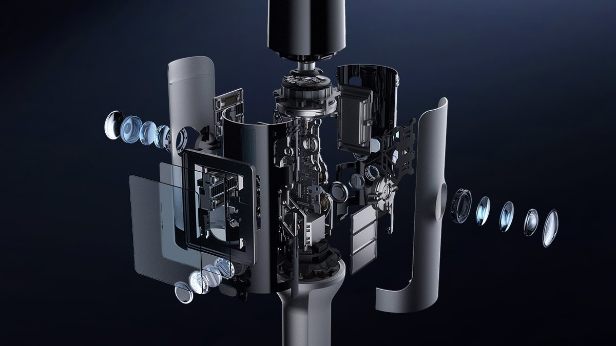
Kosmo gets poses the way survey handhelds do: lidar-inertial odometry. The IMU, sampled hundreds of times a second, predicts the motion between lidar sweeps. That prediction deskews each sweep, because the device moved while the sweep was taken. The deskewed points are then registered point-to-plane against the map, and the filter's update corrects the IMU's drift. I worked through every step of this, with code, in FAST-LIO2 from scratch.
Once the lidar trajectory exists, each camera's pose is the lidar's pose composed with a fixed calibration. That is why Hesai leads with "microsecond-level synchronization". Walking at 1 m/s, a 1 ms timing error between camera and lidar places a frame 1 mm off, and swinging the stick at 90°/s rotates it 0.09° (reasoned). At 3 m, 0.09° is 4.7 mm. Microsecond sync pushes both well under the lidar's own noise.
How lidar gets into a Gaussian splat
A 3D Gaussian splat is a few million anisotropic Gaussians, each with a position, three scales, a rotation, an opacity and a colour. Training renders them into each captured view and moves every parameter to reduce the photometric error. In the original 3DGS loss, that is a mix of L1 and D-SSIM against the photo. There are two places lidar can enter.
Initialization. Training has to start from somewhere. Photo pipelines start from SfM's sparse points, which cluster on texture and leave blank paint nearly empty. Lidar points cover the blank paint as densely as the poster on it, in metric units, in the same frame as the poses. That alone removes a whole failure class: Gaussians spawned in the wrong place on a wall SfM never triangulated.
A depth loss. Rendering a splat gives a depth per pixel as well as a colour, from the same alpha compositing:
where is Gaussian 's depth along the ray and its opacity there. Project the lidar points into the view to get a sparse reference depth , and add a term:
with the pixels that have a lidar return. Hesai has not published Kosmo Spatial Core's loss. This is the generic form, not theirs.
Why bother, if the points already seeded the right places? Niantic Spatial's post the same day answers it: "Photorealistic splats can look perfect and still hide flaws. They mask warped walls, drifting edges, and phantom bumps. Training longer makes it worse, not better." A photometric loss has many solutions. A blank wall seen from a few cameras looks the same whether its Gaussians sit on the plane or a few centimetres in front of it. Meanwhile view-dependent effects — exposure changes, gloss, a reflection — are cheaper to "explain" by nudging a Gaussian off the surface than by getting the colour right. Where texture is strong, parallax pins the depth. Where it is weak, nothing does. Without a geometric term, every extra iteration is another chance to drift (Niantic's argument; reasoned as a mechanism).
The toy below shows that mechanism and nothing more. It is not a splat optimiser. Each Gaussian on a wall feels a photometric pin, as strong as its texture and the number of views make it. It also feels a small seeded pull off the wall standing in for view-dependent colour, and, optionally, a depth term.
Start from lidar points with λ at zero and drag the training length up. The poster stays on the wall and the blank paint walks off it. That is Niantic's "training longer makes it worse": a good initialization is not enough on its own, because nothing holds it there. Any λ above zero bounds the drift. More views stiffen the photometric pin, which is why a slow, overlapping capture helps even without lidar.
How the depth term is written matters as much as having one. When Spirula Studio added LiDAR input, its depth loss was a Pearson correlation between rendered and reference depth, off by default. A correlation ignores scale and offset, so a laser's millimetres count no more than a monocular network's relative depth. A metric term, as in the equation above, is what lets lidar hold a wall at the right distance. Whether Kosmo's is metric, I cannot tell from anything Hesai has published.
Inside a real Kosmo splat
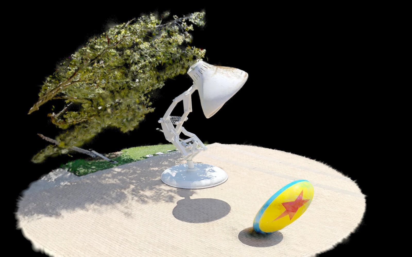
The only Kosmo output I could open is Pixar's: the plaza outside the Steve Jobs Building with the Luxo lamp and ball, scanned by Dylan Sisson with an early unit. It is 127 MB zipped, a 100.5 MB pixar-lamp-and-ball.usdc holding one ParticleField3DGaussianSplat prim. I read it with usd-core and NumPy. Everything in this section is measured on that file.
- 1,256,332 splats, matching Pixar's stated count. Each takes 80.0 bytes: positions, scales, rotations, opacities, a base colour, an estimated normal and degree-0 spherical harmonics. The file carries no view-dependent colour.
- About 14 × 7 × 12 units (0.5th to 99.5th percentile), which is a plaza if the unit is metres. The stage's
metersPerUnittag says 0.01, which would make it a 14 cm plaza. The tag is wrong, or something downstream rescales the scene. The converter in the same zip says it writes one metre per unit. - Gaussian size, one-sigma, sorted per splat: the median largest axis is 9.1 mm, the middle 3.3 mm, the smallest 1.7 mm. The 95th percentiles are 39.9, 25.1 and 14.3 mm.
- Shape: the median ratio of smallest to largest axis is 0.23, and 43% of splats are below 0.2. Most are flattened discs lying on surfaces, which is what you want for a mesh and a depth map.
- Opacity: median 0.81; 42% above 0.9 and 6% below 0.1. Few faint floaters.
One caveat: this is an outdoor plaza from a pre-release unit, exported for RenderMan by an unknown software version. It shows what one real Kosmo splat is made of, not what every capture will be.
Checking the claims
| Claim | Who says it | What is behind it |
|---|---|---|
| 569,000 pts/s, 40 m at 10%, 1535 nm, Class 1 | Hesai spec sheet | Standard spec-sheet terms; fine as stated (reported) |
| Millimetre-level geometric accuracy | Hesai press release and product page | No accuracy row in the spec; no distance, reference or control-point conditions. Plausible as local precision; unproven as global accuracy (reasoned) |
| 8K | Hesai | 8192 × 6144 fisheye frames; exports top out at 6K (Hesai's own footnote). Splats train on what is exported or processed, so detail is bounded by 6K, not 8K, unless processing reads the raw frames. Hesai does not say which (reasoned) |
| 100 m² in about 15 minutes | Hesai | "Actual capture time varies" (reported). The point budget above says it is more than enough lidar; the limit is walking every surface into camera view |
| Up to about 5x faster processing | Hesai | No baseline product, no hardware, no absolute time (reported). The Kosmo Studio manual says some stages "may take tens of minutes or several hours" locally, on a minimum of a 24 GB Ampere GPU and 64 GB of RAM (reported) |
| Dairy Queen: about 300 hours of modelling replaced by about 15 minutes, robot at 99% task success | Hesai press release | "Scanning and reconstruction took just 15 minutes", although the room-scan figure alone is 15 minutes and the manual describes multi-hour stages. Success rate has no task, trial count or baseline; "failure rate fell to one-tenth" implies about 90% before, if the 99% is the after (reasoned) |
| More than 100x the training data for the same cost | Hesai | The footnote compares RMB 10 to 20 per real-robot trajectory with RMB 0.1 to 0.2 per simulated trajectory in a Kosmo scene (reported). Real and simulated trajectories are not the same commodity |
| A lidar "tailored to Gaussian splatting", only in Kosmo | Radiance Fields | Not in Hesai's material I read. Hesai describes it only as an ultra-high-spatial-resolution lidar |
| 45-minute capture limit | Radiance Fields | Not found in Hesai's documents. Kosmo Studio caps single-scene reconstruction at 90 minutes of data and recommends 40 minutes or less on a 500 GB working disk (reported) |
Two small consistency checks pass. The standard battery is 2,900 mAh for about 60 minutes at up to 30 W. That needs about 30 Wh, so the pack runs near 10.3 V — a three-cell lithium pack, if I have guessed its chemistry right (reasoned). And the Kosmo Studio limit of about 40 minutes of capture per 500 GB of working disk is about 12.5 GB of scratch per captured minute (reasoned). Whatever the raw data rate is, local processing is not a laptop job.
Against what is already on this site
Kosmo is not the first lidar scanner that outputs splats. XGRIDS' Lixel scanners write the .lcc splat format that KOLC+ loads into BIM. The FARO and BLK360 scans in Spirula Studio's LiDAR path come from terrestrial scanners that are set down and left to spin. The cheaper route is no lidar at all: a 360 camera, SfM and a lot of overlap, as in the capture pipelines piece.
What Kosmo changes is not the idea. It is that the lidar maker builds the whole stack: emitter, scanner, sync, odometry and the splat trainer. It also brings a 1535 nm Class 1 source into a handheld. Hesai's own lidars were already inside handheld research rigs; the Hilti 2022 Phasma rig carried a PandarXT-32. Now the company sells the rig.
The outputs land in formats this site has covered. .sog is PlayCanvas's WebP-packed splat format. .ply opens in Blender 5.3. A room's lidar points are the input SpatialLM turns into a floor plan.
What I could not check
- Accuracy under stated conditions. No published spec, test, distance or reference. Nobody outside Hesai has published one either, as far as I found.
- Single-shot range noise, angular resolution and scan pattern of the lidar. The arithmetic above uses only the point rate and the field of view, and the widget treats noise as an assumption.
- Processing time. Only the "up to 5x" ratio, with no baseline, plus the manual's "tens of minutes or several hours".
- The loss Kosmo Spatial Core trains with. Whether it uses lidar depth as a metric term, a correlation, or only for initialization.
- What "6K export" covers: images, the splat's training resolution, or both.
- Price and availability: not published.
- The Dairy Queen task and trial counts.
What I take from it
The lidar numbers are generous for a room. The 569,000 points a second puts something like 150 returns inside every typical Gaussian over a 15-minute walk-through. Point density is not the bottleneck, and the spec-sheet race on point rate is not the interesting part. The interesting parts are the ones Hesai has not published: how tight the trajectory stays over a building, and whether the trainer uses the lidar as a metric constraint or just as seeds. Niantic's argument and the toy above both say seeds are not enough. The Pixar file says the output is mostly thin, opaque, surface-hugging discs, which is what a depth-constrained fit should produce. I would want a scan of a long corridor against survey marks before believing "millimetre-level" means anything beyond the room I am standing in.