Invaria: a point-cloud encoder that doesn't care what grid you sampled at

2026-10-11 · 19 min · point-cloud · 3d · lidar · robotics · benchmarks

Why read this

Why point-cloud backbones break when you change the grid, what Invaria's calibration fixes and what it can't, and what the 56% and 45% are really made of.

Original analysis
A lasting reference
A new technique

3D & spatialNothing to runResearch paper

How this was scored

Is it new?: 2 of 3: A real new idea, method or capability
Can I trust it?: 2 of 3: Measures key facts from files, code or configs
Can I run it?: 0 of 3: Closed, nothing to run
Will I understand it?: 2 of 3: Mechanism from first principles with figures
Can I act on it?: 2 of 3: A concrete recipe, numbers or comparison
Will it last?: 2 of 3: A reference for a year or more
Does it affect many?: 1 of 3: A specialist community
Only here?: 2 of 3: A teardown or measurement few others did

Score 60 of 100, ranked 270 of 494 rated articles. Each question is answered 0–3 by hand, and a 3 is rare. How articles are scored

Every LiDAR pipeline I have shipped downsamples somewhere. A voxel filter before the network, because the GPU on the robot is a quarter of the one the model was trained on, or because the latency budget is 80 ms and the scan has 200,000 points. Nobody retrains the segmentation model when they do that. They change grid_size in a config and hope.

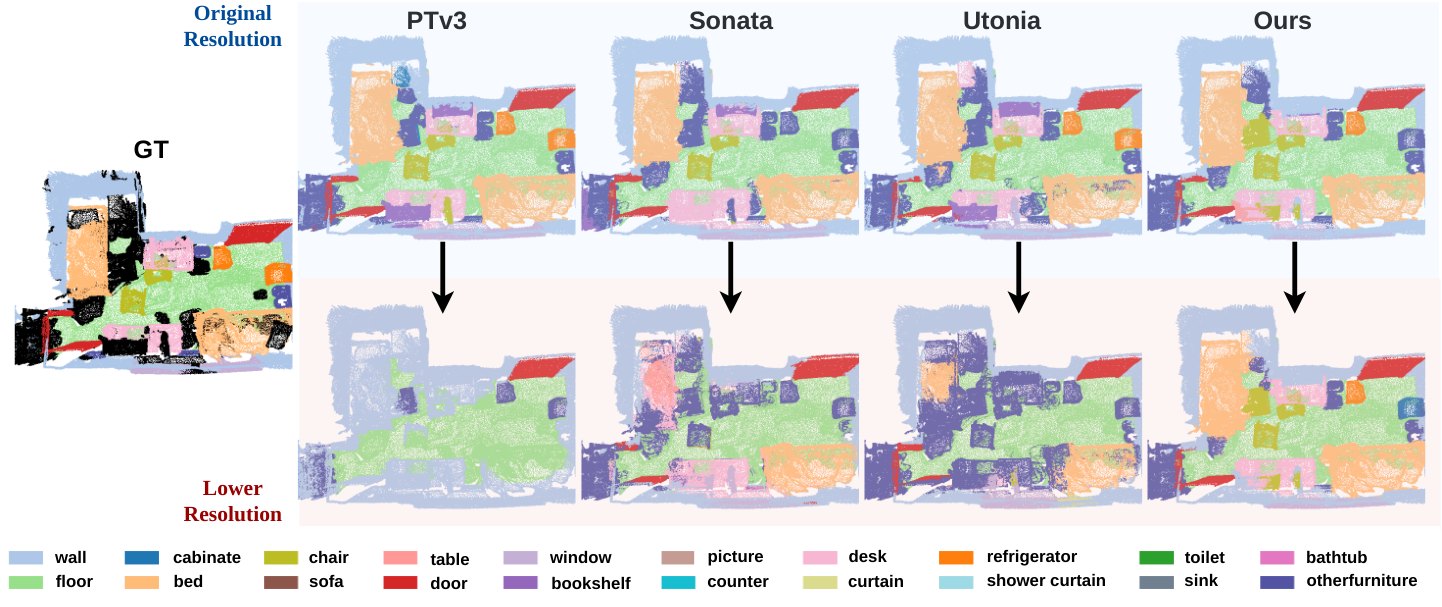
Invaria (Chun-Peng Chang, Shaoxiang Wang, Alain Pagani, Dariu Gavrila and Holger Caesar, TU Delft and DFKI; arXiv 15 May 2026, accepted at NeurIPS 2026) is a paper about what that hope costs. The number that made me read it was not theirs. It was in their Table 1, in the Point Transformer V3 row: trained on ScanNet at a 2 cm grid, PTv3 scores 77.6 mIoU at 2 cm and 20.5 at 6 cm. Three times coarser, three-quarters of the accuracy gone. Even the denser direction hurts: at 1 cm it scores 50.5.

The paper's claim is that a point-cloud encoder can be built to shrug that off, and that doing so also makes it smaller and cheaper. I read the paper end to end and the project page; the code says "coming soon", so where I quote code below it is the Pointcept implementation of PTv3 that Invaria is built on, not Invaria's own. The short version: the mechanism is real and well argued, the robustness numbers are large, and the comparison is set up in a way you should understand before you quote the 56%.

The grid size is a unit of measurement

Start with what a modern backbone does to a point cloud before any learning happens. In Pointcept, which hosts PTv3, Sonata, Concerto and Utonia, the GridSample transform divides every coordinate by the grid size and floors it:

# pointcept/datasets/transform.py:864-865 (Pointcept @ 1342eda)
scaled_coord = data_dict["coord"] / np.array(self.grid_size)
grid_coord = np.floor(scaled_coord).astype(int)

From that point on, the network mostly lives in grid_coord. The sparse convolutions count their kernels in cells: the stem is a SubMConv3d with kernel_size=5 (point_transformer_v3m1_base.py:506-509), and every block's positional encoding is another with kernel_size=3 (:285-288). Pooling right-shifts the serialized code and the grid coordinates by the stride (grid_coord=point.grid_coord[head_indices] >> pooling_depth, :429). The Pointcept README even notes that replacing precise coordinates with grid coordinates doesn't hurt accuracy, which is true right up until somebody changes the grid.

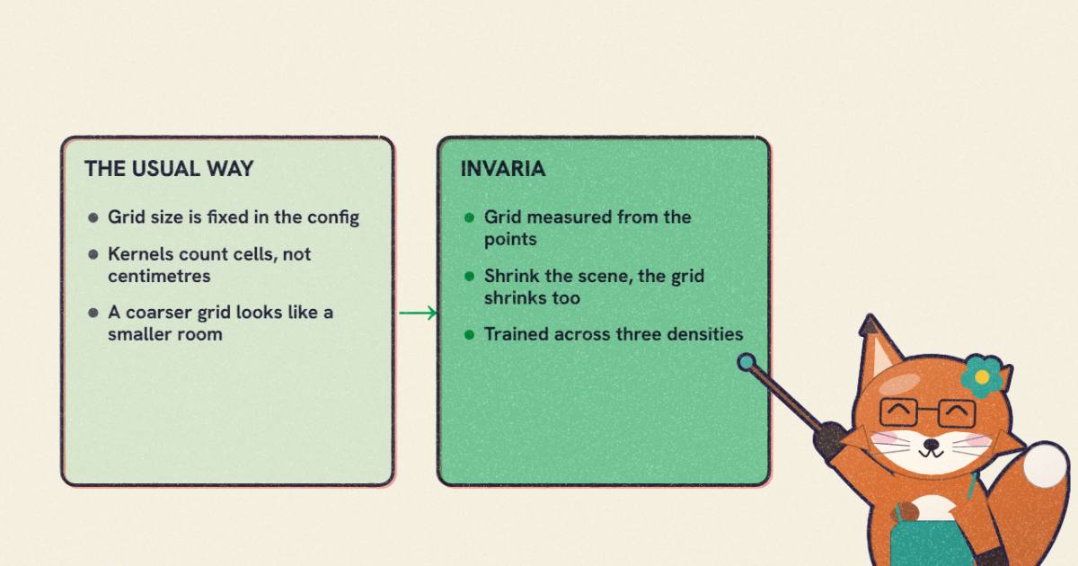
So a 3×3×3 kernel at 2 cm reaches 6 cm of chair. At 6 cm it reaches 18 cm. The paper writes this as a generic neighbourhood aggregation, where an operator $\Omega$ pools the features within a fixed kernel $\mathcal{K}$ of grid distance:

\mathcal{F}_c = \Omega\left(\left\{ f_i \;\middle|\; \frac{d(c,i)}{\tau} \le \mathcal{K} \right\}\right)

The division by $\tau$ is the whole problem. Tripling $\tau$ is, from inside the network, the same as shrinking every object in the room to a third of its size. The model was never shown a 15 cm chair, so it doesn't find one.

Their second failure mode is density, and it bites the operators that count points rather than cells. A $k$ -nearest-neighbour group always has $k$ members, so its physical reach grows as the cloud thins: the paper's Eq. 8 puts the reach at $\mathcal{R} \propto \tau \cdot \sqrt[3]{k}$ . PTv3's serialized attention is the same story in a different costume. Its patches are 1,024 consecutive points along a space-filling curve (enc_patch_size=(1024, …) in configs/scannet/semseg-pt-v3m1-0-base.py:23), so a coarser cloud packs a bigger chunk of the room into every attention window. A ball query with a fixed metric radius goes the other way: the reach is fixed and the number of points inside it collapses.

These are the same ingredients behaving in opposite directions, which is easier to see than to read. The toy below is a side view of a room, grid-sampled at the $\tau$ you pick, with a query point on the chair seat.

one neighbourhood, four operators · toy 2D sceneillustrative geometry

points inside

physical width

24.0 cm

share of chair seen

52%

grid size τ2.0 cm

scene scale (same points)

The reach never moves, so the count tracks the density: push τ from 2 to 6 and the seat's neighbourhood loses more than half of its points.

Push the grid from 2 cm to 6 cm with the ball selected and the seat's neighbourhood loses more than half its points; the reach doesn't move. Switch to k-NN and the count is pinned while the circle swells. Switch to the 5×5 grid kernel and it spans 22% of the chair's width at 2 cm and 65% at 6 cm. Then leave $\tau$ at 2 and shrink the scene to a third: the grid kernel now spans 65% of the chair again. That coincidence is the paper's point. A coarser grid and a smaller object are the same event to a grid-native network.

One detail in the paper's appendix is off, and it matters for intuition. Appendix D says tripling $\tau$ should cut the point count by $3^3$ , 27-fold. That holds for a filled volume. A depth sensor or LiDAR samples surfaces, and a surface sampled on a 3× coarser grid loses closer to $3^2$ , about 9-fold, of its points. In the 2D toy the scene is made of lines and the count drops with $\tau$ to the first power: 481 points at 2 cm, 158 at 6 cm. The ScanNet clouds in the test are thinner than the baseline's training data, but not by 27×.

A ScanNet bedroom segmented by four models. The top row, at the original resolution, shows PTv3, Sonata, Utonia and Invaria all colouring the bed orange, chairs olive, desks pink and the floor green. The bottom row, at lower resolution, shows PTv3 painting almost everything as wall or floor, Sonata smearing a pink table label across the bed, Utonia turning much of the room purple as other furniture, and Invaria still showing the bed, desks and chairs much as before. — Same scene, same weights, two input resolutions. The baselines were trained at the default grid and evaluated at a coarser one; the bed and desks are where PTv3 and Utonia give up. (Invaria paper, Figure 2.)

What Invaria changes

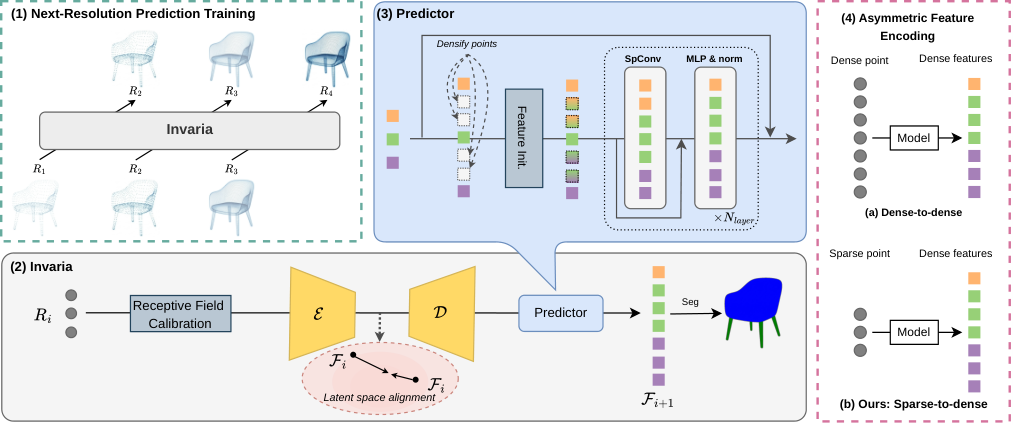
The paper's own framing is three components: receptive field calibration, next-resolution prediction, and a latent alignment loss. Having read them, I think the cleanest way to hold them in your head is that the first one is a measurement and the other two are training pressure. The measurement fixes scale. The pressure has to fix density.

Measure the grid instead of declaring it

Receptive field calibration throws out the configured grid size. Given a cloud $\mathcal{P}$ of $N$ points, it draws $N_a$ random anchors, finds each anchor's distance to its nearest distinct neighbour $d_i$ , and sets the internal grid to

\psi(\mathcal{P}) = \alpha \cdot \rho\left(\{d_i\}_{i=1}^{N_a}\right)

where $\rho$ is a reduction and $\alpha$ a constant. Algorithm 1 in the appendix is exactly this, eight lines long. The appendix also explains why $\rho$ is the mean rather than the minimum, and it is the kind of detail that tells me somebody tried it. The minimum looks principled, because every pair of points should land in separate cells. But anchor distances are measured between arbitrary positions, not cell centres; with 26 neighbouring cells in 3D, two points either side of a shared face or corner can be nearly touching, so the minimum comes out far too small.

Calibration buys one thing completely and another not at all. If the whole scene shrinks by 3× and keeps its points, every nearest-neighbour distance shrinks by 3×, the measured grid shrinks by 3×, and the grid coordinates come out identical. Scale invariance by construction. Pick "calibrated grid" in the toy and step through the three scales: the share of chair the kernel sees doesn't move.

Now leave the scale alone and resample at 6 cm instead of 2. The mean nearest-neighbour distance is now about 6 cm, the measured grid is about 6 cm, and the grid coordinates are exactly as coarse as the baseline's. Calibration gives a resolution shift no help at all. Whatever robustness Invaria shows at 6 cm has to come from training.

The ablations agree. Without calibration (Table 6a) Invaria still scores 69.7 at 6 cm, but falls to 55.7 at 1 cm. Without next-resolution prediction (Table 6b) it collapses at the coarse end, to 21.7 at 4 cm and 9.5 at 6 cm, which is worse than plain PTv3. So: training does the heavy lifting on resolution, and calibration mainly rescues the denser-than-training direction, where a declared 2 cm grid would otherwise misjudge a 1 cm cloud.

Predict the next resolution up

Training sees each scene at several densities. On ScanNet the appendix gives the subset sizes as $n_0 \cdot h^i$ with $n_0 = 4096$ and $h = 4$ , so 4,096, 16,384 and 65,536 points. The model takes the sparser one, encodes it with a PTv3-style U-Net, and a small predictor densifies: it adds points at the next resolution's real coordinates (or interpolated ones when there are none), seeds their features from the nearest encoded point, and refines them through a few blocks of sparse convolution, MLP and norm. The loss is segmentation (cross-entropy plus Lovász-softmax) on the predicted features at the next resolution, summed over levels with weights that grow toward the finest (Table 6d found increasing weights slightly better than uniform):

\mathcal{L}=\sum_{m=1}^{M-1}\lambda^{(m)}\left(\mathcal{L}_{\text{CE}}+\mathcal{L}_{\text{LS}}\right)+\beta\,\mathcal{L}_{\text{align}}

The inspiration they cite is next-scale prediction in image generation, VAR and Infinity. The point is not to generate points. A model that must produce correct labels for a denser cloud than it was given cannot get away with features that only work at one density.

The alignment term pairs each bottleneck token at one resolution with its spatially nearest token at another and minimises cosine distance between them. It is the least important of the three: removing it (Table 6e) costs between 0.5 and 0.8 points at every resolution.

The Invaria framework in four panels. Panel 1 shows a chair at resolutions R1 to R4, with Invaria taking each resolution and predicting the next. Panel 2 shows the pipeline: input points at resolution Ri pass through Receptive Field Calibration, an encoder E and decoder D with a latent space alignment loss between bottleneck features, then a Predictor, producing features at resolution i+1 and a segmentation. Panel 3 expands the predictor: points are densified, features initialised, then refined through repeated sparse convolution and MLP-and-norm blocks. Panel 4 contrasts dense-to-dense encoding with Invaria's sparse-to-dense encoding, where a few input points produce dense output features. — The training objective (top left), the encoder with calibration and alignment (bottom), the predictor that densifies features (top centre), and the sparse-to-dense inference that the token savings come from (right). (Invaria paper, Figure 5.)

Where the smaller model and the fewer tokens come from

Two efficiency claims ride along: a 45% smaller model and 40% fewer input tokens. They have different origins and different amounts of evidence.

The model size is the easy one. Invaria's encoder, per Appendix B, has stage depths (2, 2, 2, 2, 1) with channels (32, 64, 128, 256, 512). PTv3's ScanNet config has depths (2, 2, 2, 6, 2) with the same channels and heads (semseg-pt-v3m1-0-base.py:20-22). The decoder is identical. So Invaria is PTv3 with four blocks removed from the 256-channel stage and one from the 512-channel stage.

I counted what that is worth from the Block definition in Pointcept. Each block holds a 3×3×3 sparse convolution plus a linear layer as positional encoding, the qkv and output projections, and an MLP with ratio 4: about $40C^2$ parameters at width $C$ . Four blocks at 256 channels come to about 10.5M, one at 512 another 10.5M, so roughly 21.0M of PTv3's 46.1M. The paper's two models differ by 20.6M (46.1M against 25.5M), which leaves a few hundred thousand parameters for the predictor. The "45% smaller" is 25.5 against 46.1, and it is a shallower PTv3. I think it's a sound design choice: Table 6f shows one bottleneck layer scoring 76.2 against two layers' 76.0. It just isn't a new kind of efficiency, and the 45% is measured against the smallest transformer in the table. Against the 39.2M sparse-conv UNet it is 35%.

Invaria-s goes further by swapping in the LitePT design, which keeps attention to the deep stages and uses convolutions early: 16.3M parameters. Appendix B calls its FLOPs saving "~7%"; Table 3 lists 230 GFLOPs against Invaria's 267, which is a 14% saving. One of those is a typo, and I can't tell which.

The token claim is the one I'd most like to see a table for. The mechanism is the asymmetric inference in panel 4 above: because the model was trained to produce dense features from a sparse input, at test time the U-Net encodes a subsample and the predictor fills in the rest. Fewer points into the transformer stages means fewer tokens, and attention cost grows with tokens.

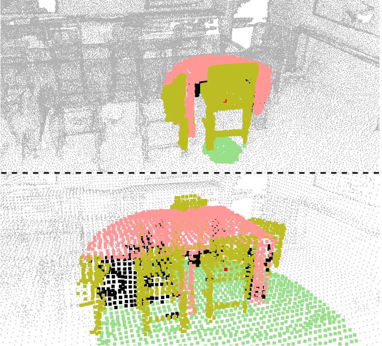
A chair in a ScanNet room, shown twice. In the top view, at high resolution, the coloured region marking one operator's receptive field covers only part of the chair and table. In the bottom view, at lower resolution, the same operator's coloured region covers the whole chair, the table beside it and a wide patch of floor. — The same operator at two resolutions: the denser input (top) sees a smaller part of the scene. The paper uses this to argue that feeding the encoder a sparser cloud is not only cheaper but can help. (Invaria paper, Figure 6.)

The paper also argues that sparser input is better for the encoder, not just cheaper, because a fixed- $k$ operator on a dense cloud sees too little of the room. Figure 6 makes the case visually and PTv3's 50.5 at 1 cm makes it numerically. But the "average reduction of around 40%" appears in the abstract, the introduction and one sentence of Section 4, and nowhere as a measurement. The appendix says the inference subset sizes are "scaled relative to the input scene size" without giving the ratio. Table 3's FLOPs (267 G for Invaria, 352 G for PTv3) don't state the input size either, so I can't tell whether they already include the subsampling. I couldn't verify the 40%.

Reading the evaluation

The two robustness tests, side by side, with every number from Tables 1 and 5. Toggle between them.

ScanNet val mIoU as the input drifts · trained at 2 cm

at the right edge, against Utonia

73.8 vs 47.3: +56.0% relative, +26.5 points

at the training setting (middle-left)

Invaria 76.2 · PTv3 77.6 · Concerto-L 78.6

Dashed: self-supervised models scored by linear probing on the authors' released weights. Solid: trained on ScanNet at 2 cm. Hover a line to isolate it.

What the 56% is

The abstract says Invaria "achieves a 56.0% higher mIoU at 3× lower resolution". The column is $3\tau^*$ , a 6 cm grid. The best baseline there is Utonia at 47.3; Invaria scores 73.8. 73.8 / 47.3 is 1.560, so the 56.0% is a relative gain over the strongest competitor, and the absolute gap is 26.5 mIoU points. Against PTv3 at 20.5 it would be a 3.6× ratio, so they chose the conservative comparison, which I appreciate.

The scale claim, "a 20% improvement when the objects scale is reduced by a factor of 3", is Table 5's ×1/3 column: Invaria 73.8 against Concerto-L 61.4, a 1.20 ratio and 12.4 points. Given what calibration does to a pure rescale, I'd have expected Invaria's scale curve to be flat by construction, and it is: 73.8 to 76.2 across a 6× range of scales. The flatness is the mechanism working as designed.

Who was trained on what

This is where you have to read the footnotes. Every baseline was trained at the 2 cm default and nothing else. Invaria was trained at three densities, a 16× spread in point count. It would be strange if a model trained across densities didn't beat models trained at one.

The authors know this and run the obvious control: PTv3 with resolution augmentation. It loses 2 points at the training resolution (77.6 to 75.6), and when tested at 1 cm, outside its augmented range, it drops to 56.0. The paper sets that against Invaria's 76.2, which is its default-grid score; at 1 cm Invaria scores 75.5, so the point stands. (That 56.0 is a coincidence with the headline; it's a different number.) I'd have liked that augmented PTv3 as a row in Table 1 at all four resolutions, because it is the baseline a practitioner would actually reach for. As it is, it's one sentence of prose.

The three self-supervised models, Sonata, Concerto-L and Utonia, are scored by linear probing on the authors' released weights: frozen encoder, one linear layer trained on top. It's a legitimate way to measure the representation, but Pointcept ships decoder-probe and full fine-tune configs for all three, and a fine-tuned head might degrade differently. PTv3's 77.6 matches, to the decimal, the ScanNet val number in Pointcept's model zoo, which suggests they used the released checkpoint there too.

Then there is Figure 7, which I think is the most honest figure in the paper and the one that most complicates the headline.

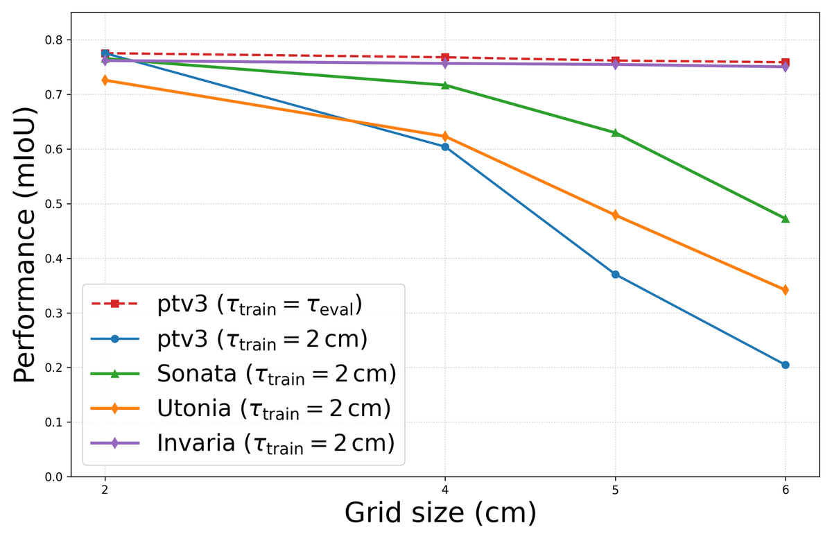
A line chart of mIoU on ScanNet against grid size at 2, 4, 5 and 6 cm. A red dashed line for PTv3 trained and evaluated at the same grid stays flat near 0.77 to 0.76. A purple line for Invaria trained at 2 cm stays flat just below it, near 0.76 to 0.75. Lines labelled Sonata (green), Utonia (orange) and PTv3 trained at 2 cm (blue) all fall as the grid coarsens, PTv3 lowest at about 0.2 at 6 cm. — PTv3 retrained at each grid (red, dashed) against models trained at 2 cm only. A cloud at 6 cm still carries enough geometry for about 76 mIoU, if the model is trained for it. The green and orange legend entries appear to be swapped: the green line matches Table 1's Utonia numbers and the orange one Sonata's. (Invaria paper, Figure 7.)

The red dashed line is PTv3 trained at each resolution and tested there. It stays around 76 at 6 cm, which is the paper's evidence that the information is still in the cloud and the baselines are taking a shortcut. It is also evidence of something else: a PTv3 retrained at 6 cm scores higher at 6 cm than Invaria does (I read about 76 off the plot; Table 1 has Invaria at 73.8). If you know your deployment resolution and can afford a training run, retraining the baseline wins. Invaria's case is the deployment where you can't: one checkpoint for every sensor, every voxel filter, every latency budget.

Two small things I measured off that figure. The green and orange markers sit at 71.5 and 62.3 at 4 cm, and at 47.1 and 34.2 at 6 cm, which are Table 1's Utonia and Sonata values with the labels exchanged. And Invaria's purple marker at 6 cm reads about 75.0, where Table 1 says 73.8. Neither changes a conclusion. Table 4 has a similar slip: its Concerto-L row of "relative drops" is printed positive (Toilet +96.2%) while every other row is negative.

At the resolution you trained for

Read the second column of Table 1 on its own and Invaria is not the best model in it. At the default 2 cm grid the order is Concerto-L 78.6, PTv3 77.6, Utonia 76.6, Invaria 76.2, the sparse-conv UNet 75.6, Invaria-s 73.3 and Sonata 72.6. Fourth of seven, 1.4 points behind the model it is built from. On nuScenes at the 5 cm default (Table 2) the gap is wider: 76.2 against PTv3's 80.4. Away from the default Invaria wins everywhere, by a lot; at it, you pay a little. The abstract's "maintaining high efficiency" is accurate; I wouldn't call the default-resolution result competitive with the state of the art, and the paper mostly doesn't either.

The test where the margin disappears

Appendix Table 7 is the one I'd send to anyone who wants to use this. It changes density without changing the grid: random subsampling to 10% and 5% of the points, coordinates still on the 2 cm lattice. At 10%, Invaria scores 64.0. Concerto-L scores 65.4, Utonia 63.9, PTv3 61.7. At 5% Invaria leads, 48.2 against Utonia's 41.8, but everyone is far below their 2 cm score.

Two things follow. First, Invaria's advantage under a pure density cut is much smaller than under a grid change. Second, and more useful: PTv3 holds 61.7 at 10% random density but drops to 20.5 when the grid goes to 6 cm, a change that thins the cloud by a similar order of magnitude. Most of the baseline collapse in Table 1 is the grid-unit effect from the first section, the model seeing a shrunken room, rather than missing points. Which suggests a cheap thing to try on a baseline you already have: downsample however you need to, but compute grid_coord at the grid size the model was trained on. I haven't tested that, and on a sparse-convolution model the empty cells will hurt, but Table 7 says it should recover a large share of what Table 1 shows being lost.

What isn't out yet

The project page links "Code (coming soon)". There are no weights, so nothing here can be run, and a few numbers I'd need to reproduce the method aren't in the paper: the anchor count $N_a$ , the scale constant $\alpha$ , the alignment weight $\beta$ , the per-level weights $\lambda^{(m)}$ , the number of predictor blocks, the subset ratio used at inference, the input size behind Table 3's FLOPs, and training time. Training used two A100 80GB cards; evaluation one. The ScanNet results are on the 20-class val split; nuScenes is the only outdoor set, and the self-supervised baselines appear there only at the default grid.

Would I use it

For a fixed sensor and a fixed preprocessing chain, no: retrain PTv3 at your resolution, or fine-tune Concerto, and you'll beat it at that one setting. For a perception stack that runs one model across sensors with different densities, or downsamples adaptively to hit a latency target, Invaria is the first thing I've read that treats the grid as something to measure rather than a constant baked into training. Calibration alone is worth stealing: it is a few lines, it makes metric scale a non-issue by construction, and nothing about it is specific to their training recipe.

The broader point I'll keep is the one the paper makes quietly. A grid-native point-cloud network does not see centimetres. It sees cells, and the config file decides how big a cell is. Every time you change that number, you have shown the model a different world.

If you work on the LiDAR end of this, the odometry side has the same sensitivity to point density in different clothes: FAST-LIO2 and FAR-LIO both voxel-downsample before registration and tune that filter by hand. For a scene representation that is resolution-free by design rather than by training, see Surflo. And the first 3D reconstruction roundup is a companion on reading benchmark tables for what they were measured on.

Pointcept/Pointcept@1342eda · snapshot 2026-10-11

tracked files

617

license: MIT
branch: main
tests: 9 files
source: 4.8 MB
commit date: 2026-09-11

source by language

Python4.6 MB(508)CUDA100.8 kB(21)C++57.8 kB(25)C28.3 kB(22)Shell20.6 kB(15)

by size of tracked source at this commit, file counts in brackets; docs, data and vendored trees excluded

local clone, 2026-10-11 at 1342eda — branch, commit, commitDate, fileCount, hasTests, languages, license, licenseFile, shallow, testFileCount

shallow clone: counts describe the pinned tree, not the history

How I checked

I read the arXiv HTML of 2605.15923v1 in full, including the appendix, and the project page; the LinkedIn post linked from the X thread is where both links came from. The code isn't released, so I shallow-cloned Pointcept at 1342eda and read the PTv3 model, the GridSample transform and the ScanNet config for the grid-coordinate behaviour, the baseline depths and the parameter count. The 56.0% and 20% are recomputed from Tables 1 and 5; the model-size breakdown is my count of a PTv3 block ( $40C^2$ plus norms and biases) times the blocks Invaria removes. The Figure 7 readings come from locating the coloured markers in the original 3000-pixel plot and mapping them to the axis, good to about ±0.3 mIoU. The toy is my own 2D geometry, not the paper's data.