2026-10-15 · 17 min · 3d · gaussian-splatting · creative-tools · gpu
Why read this
Hightop 30%Reads Blender 5.3's splat code engine by engine: hashed alpha in EEVEE, a stochastic hit in Cycles, and why depth of field works with no special case.
- Interactive explanations
- Original analysis
- Runs on a consumer GPU
3D & spatialGPL-2.0-or-laterPractitioner tool
How this was scored
- Is it new?
- 2 of 3: A real new idea, method or capability
- Can I trust it?
- 2 of 3: Measures key facts from files, code or configs
- Can I run it?
- 2 of 3: Open code or weights with real limits
- Will I understand it?
- 3 of 3: Mechanism carried by interactives built from real code or data
- Can I act on it?
- 2 of 3: A concrete recipe, numbers or comparison
- Will it last?
- 2 of 3: A reference for a year or more
- Does it affect many?
- 2 of 3: A widely used model, tool or lab release
- Only here?
- 2 of 3: A teardown or measurement few others did
Score 74 of 100, ranked 65 of 577 rated articles. Each question is answered 0–3 by hand, and a 3 is rare. How articles are scored
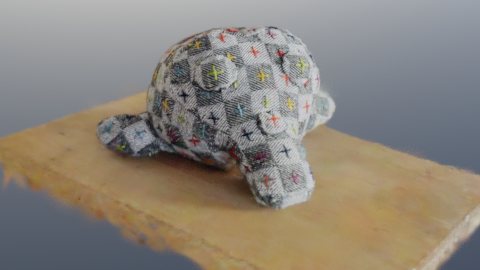
On 14 October, KIRI Engine posted a short clip of one of its phone scans opened in Blender 5.3: "Not only does Blender 5.3 add native GS support, but depth of field also works." They used an orthographic camera with a very shallow focus, and a church tower came out looking like a model railway. One reply said exactly that.
That is not free. A standard 3DGS renderer sorts 2D ellipses and blends them; it never casts
a ray. I read the blender-v5.3-release branch at commit 3ed5b28, the
5.3 rendering release notes
and the pull requests, to see what Blender does instead. I did not run Blender. Numbers are
measured (I computed them, some from 100,000 splats of a real scene), reported
(Blender's own text) or reasoned (my arithmetic on the other two).
What shipped, and when
The groundwork is PR !163102, "Integration of gaussian splats for IO and rendering", by Sergey Sharybin. It merged on 16 September 2026 with 7,951 lines added across 217 files (reported). The engines came in !163103 (Cycles) and !163367 (EEVEE, Workbench, overlays); geometry nodes in !163530 and !163624.
The 5.3 milestone puts beta on 30 September, the release candidate on 4 November and the release on 10 November 2026 (reported). The release notes say "There is currently no export support"; I found no writer for either format.
Where a splat lives: a point cloud with a type
A 3DGS splat is a 3D Gaussian. It has a centre, three scales along its own axes, a rotation,
an opacity, and a colour that changes with view direction, stored as spherical-harmonic (SH)
coefficients. Blender did not add a new object type for this. It added a Type enum to the
existing PointCloud data-block, with two values: Points (the old behaviour) and
3D Gaussian Splats. The splat fields become named attributes on the points:
| attribute | type | holds |
|---|---|---|
position | float3 | the centre (the point cloud's own positions) |
scale | float3 | standard deviations along the splat's axes, in object units |
rotation | quaternion | the splat's orientation; the PR notes it is "not guaranteed to be normalized" |
radiance:base | float4 | the SH DC term in xyz, opacity in w |
radiance:sh_0 … radiance:sh_N | float3 each | SH coefficients for bands 1 and up, in order L=1 M=-1, L=1 M=0, L=1 M=1, L=2 M=-2 … |
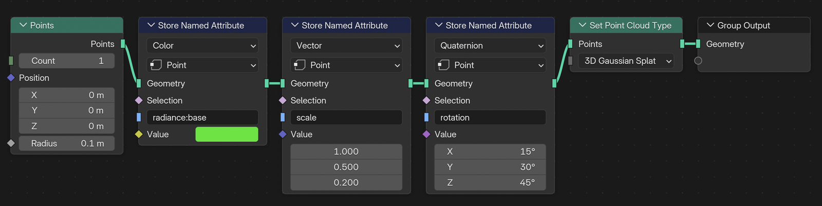
Because these are ordinary attributes, geometry nodes can make a splat from nothing. The screenshot in !163530 does exactly that: one point, three Store Named Attribute nodes and a Set Point Cloud Type node.
A file does not store these values the way Blender does. The original 3DGS trainer saves the
values from before its activation functions, because that is what it optimizes. Blender's
PLY importer undoes this per splat, in ply_import_gsplat.cc and IO_gsplat.hh:
- scale:
exp(), since the file holds log standard deviations; - opacity:
1 / (1 + exp(-o)), a sigmoid, clamped to 0..1; - rotation: normalized, after reading
rot_0..3asw, x, y, z; - SH bands 1+:
f_rest_*is stored channel-major (all of red, then green, then blue), and Blender regroups it into one float3 per coefficient; - DC colour: kept as an SH coefficient. It turns into a colour only at render time, as
0.2821 × f_dc + 0.5, and that result is treated as sRGB and converted to linear.
Here is one real splat, vertex 542,403 of the bonsai scene (measured). Each toggle is one conversion; the dashed circle is the bounding sphere Cycles builds for it (below).
As stored, this splat has log-scales of −4.93, −6.34 and −4.77, an opacity logit of 2.02 and a quaternion of length 1.054. After conversion it is a flat ellipsoid measuring 7.23 × 1.77 × 8.48 mm at one sigma, with opacity 0.883, and a DC colour of sRGB (0.524, 0.665, 0.787), which is linear (0.237, 0.400, 0.582). All reasoned: Blender's formulas on the stored floats. The quaternion length matters: across 100,000 splats of the scene the median is 0.9599, the 5th to 95th percentile 0.784 to 1.297 (measured). The trainer normalizes before use and stores the raw value, so an importer that skips this skews millions of splats.
Which SH degree survives
Import goes higher than render. PLY and SPZ both import up to degree 4 (72 f_rest
properties); every renderer stops at degree 3.
- Cycles packs bands 1 to 3 into a 45-byte
PackedSphericalHarmonicsRest: 15 coefficients × 3 channels, each mapped from −1..1 onto one byte. Degree 4 was dropped as "probably barely perceivable". - EEVEE, Workbench and the overlays pack degrees 0 to 3 into 48 bytes, and the shape (22-bit
centre per axis, 9-bit scales and rotation, 8-bit opacity) into a 16-byte
uint4.
So the viewport holds 64 bytes per splat against 248 in a degree-3 float PLY: 79.7 MB of GPU buffers for the 1,244,819-splat bonsai scene, against a 308.7 MB file (reasoned). An 8-bit SH step is 2/255 = 0.0078, and no bonsai coefficient nears the ±1 clamp; the largest is 0.861 (measured). For the SH budget see 192 bytes of spherical harmonics, or 28 bytes and a tiny MLP; for a compressed on-disk format, SOG.
Getting splats in: PLY, SPZ, and which way is up
PLY. A file is a splat when it has no edges, faces or UVs and all of f_dc_0..2,
opacity, scale_0..2 and rot_0..3 exist; zero vertex normals (which spz_to_ply writes)
are tolerated. The Import PLY node runs the same check, hence its output's rename from Mesh to
Geometry.
The axes are the trap. Splat PLYs use COLMAP's +Z forward, −Y up, as the notes say, but the
importer still defaults to Blender's Y forward, Z up (io_ply_ops.cc), and the conversion is an
object matrix. Import with defaults and the scan lies on its side; set Forward = Z and Up = −Y
yourself. The geometry node has no axis option at all.
SPZ. Niantic's compressed format gets its own reader in source/blender/io/spz: gzip
containers for versions 2 and 3, Zstd streams for version 4. The PR chose its own code over
Niantic's library for memory, and because glTF will later need a v2 writer. SPZ is right, up,
back, so every splat is rotated +90° about X: positions become (x, −z, y), the quaternion is
pre-multiplied, and each SH band is rotated with closed-form matrices adopted (MIT) from
Niantic's library. The decoding:
- colour is
(byte / 255 − 0.5) / 0.15, deliberately a smaller scale than the 0.2821 DC constant, so the DC term can overshoot and the higher bands can pull it back; - scale is
exp(byte / 16 − 10); - opacity is
byte / 255directly (the sigmoid and its inverse cancel, and the code keeps both for reference behindif (false)); - the v3+ quaternion is "smallest three" at 10 bits each plus a 2-bit index.
USD and glTF. The Pipeline & I/O notes add readers for USD's
UsdVolParticleField3DGaussianSplat schema and for glTF splats. No exporters.
How each engine draws a splat
The original 3DGS renderer sorts. It projects every Gaussian to a 2D ellipse, sorts the ellipses per screen tile by depth and alpha-blends them front to back. Blender 5.3 sorts nowhere. Each engine replaces the sort with something that gives the right answer on average over samples.
Workbench: a dithered cut-out
Workbench's opaque pass evaluates the 2D Gaussian per fragment and discards it when the alpha falls below a hash of its position; X-ray mode uses weighted blended order-independent transparency. It is fast, it shimmers, and it is fine for blocking out a shot.
EEVEE: project, then hash the alpha
A compute prepass (draw_gsplat.bsl.hh) runs once per splat per view:
- Cull splats behind the camera, below 1/255 opacity (the 3DGS paper's threshold, which trained data assumes), with a zero or NaN scale, or off screen.
- Project the covariance
R S Sᵀ Rᵀto 2D with the EWA Jacobian, which has an orthographic variant. The 3DGS 0.3-pixel low-pass is commented out: it "better matches Cycles". - Emit a billboard quad along the 2D axes, and evaluate SH degrees 0 to 3 for the view.
Then, in the depth prepass, each fragment computes exp(−d²) × opacity and is discarded if
its transparency exceeds a hashed threshold that changes every EEVEE sample. A survivor is
opaque, writes depth and is shaded like any surface; averaged over samples, the result
converges to the blend. It is EEVEE's existing hashed alpha, applied to every splat.
Cycles: a primitive you can hit
This is the interesting part. A path tracer needs an answer to "what does this ray hit,
and where", and a Gaussian has no surface. Cycles answers with three steps, all in
intern/cycles/kernel/geom/gsplat_intersect.h.
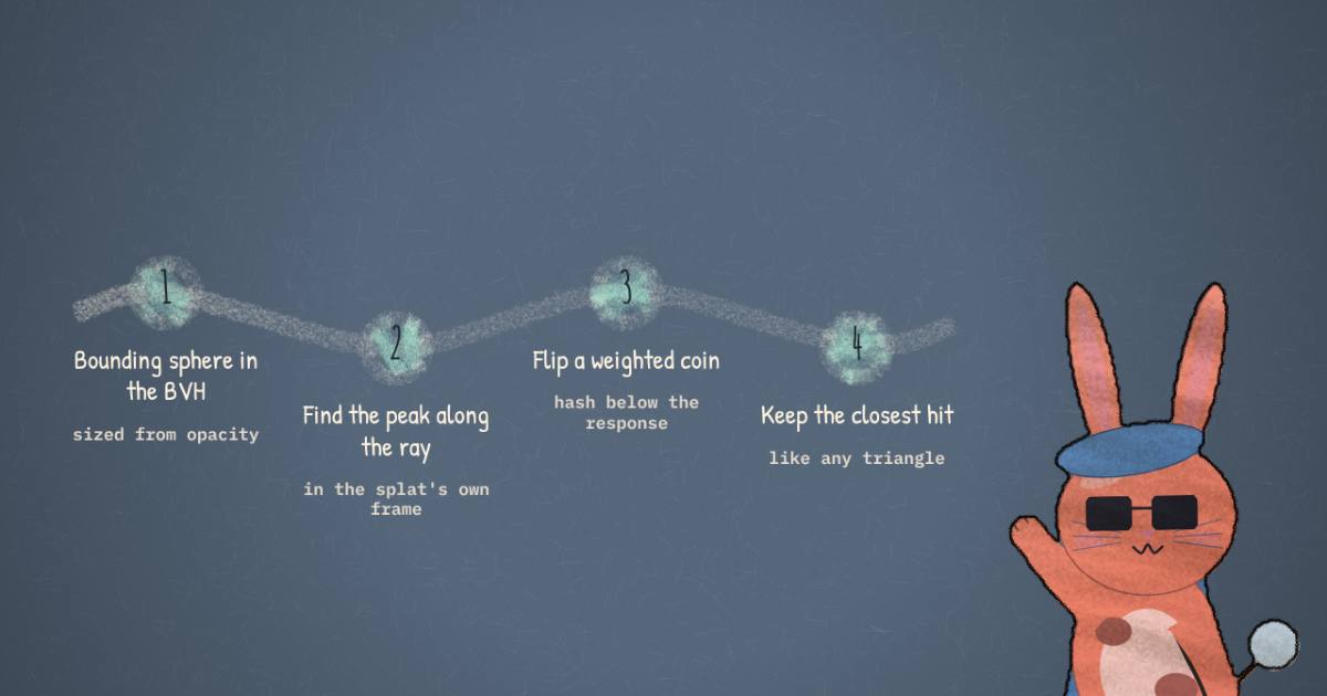
A bounding sphere for the BVH. Splats go into the BVH as points, and the sphere radius is
computed at sync time from the splat's own opacity and scale
(PointCloud::update_gsplat_radii, following
3DGRT, Eq. 7):
That is the distance at which a Gaussian of peak opacity falls to a response of 0.01. At the factor is sigma (reasoned). On bonsai the median factor is 2.64 and the maximum is 3.035 (measured). A splat with below 0.01 gets radius 0, so no ray ever hits it.
The point of peak density along the ray. Inside the sphere, the kernel moves the ray into the splat's own frame with , where the Gaussian becomes a unit sphere. It then takes the closest approach:
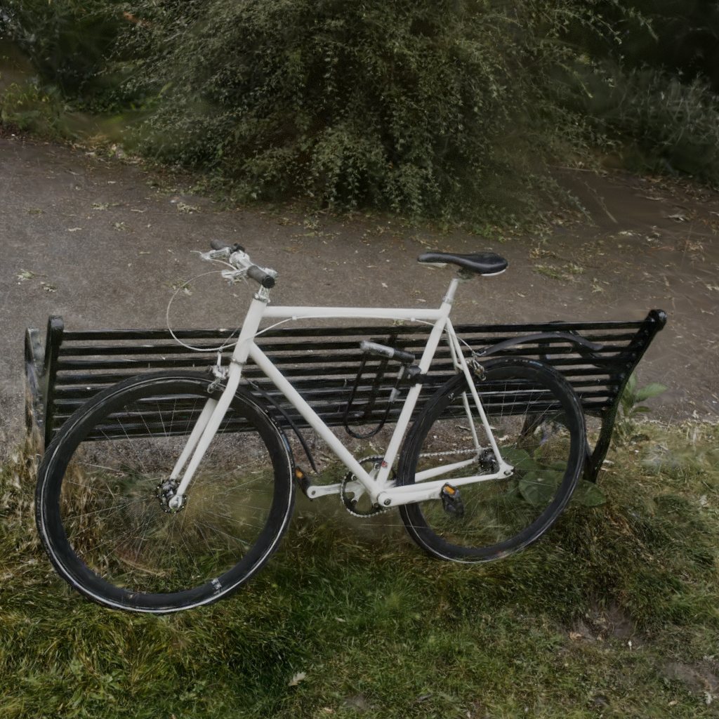
At the point , the response is . The code keeps a commented-out "naive" version that builds directly. Its comment says that version turned the near-transparent floaters in the bicycle and garden scenes into "large almost opaque spheres", from loss of precision.
A coin flip instead of a sort. Then comes Sun et al., "Stochastic Ray Tracing of Transparent 3D Gaussians" (EGSR 2025): hash the hit position to a number in 0..1 and accept the hit only if the number is below that response. An accepted hit is an ordinary, opaque intersection, so the BVH keeps the closest accepted one, as it would for triangles. Splat i wins only if it is accepted and every splat in front of it is rejected, so it wins with probability . That is exactly the weight front-to-back compositing would give it. Over many samples per pixel the expected colour is the composited colour, and nothing was ever sorted. The paper's abstract claims the cost of rays through a splat asset "is comparable to that of standard mesh-intersection rays" (reported; I did not measure Cycles).
The demo uses four made-up alphas: 0.35, 0.6, 0.25 and 0.9. The compositing weights are 35%, 39%, 6.5%, 17.6% and 2.0% for the background (reasoned). Trace a few thousand rays, and the observed shares and the averaged colour settle onto those weights. That holds whether or not the splats are visited in random order.
Since the hit is a real intersection, the rest of Cycles works on it. The PR checklist ticks off motion blur. Shading happens at a point, so a splat needs a normal for any BSDF. Cycles takes the splat's shortest axis, following PGSR's "flattening" argument: a flat Gaussian is a small disc. EEVEE builds its billboard normal the same way.
Where the two engines will disagree
- 2D versus 3D. EEVEE evaluates the Gaussian after projecting it (EWA); Cycles evaluates the 3D Gaussian at its peak along each ray. They agree for small, distant splats and diverge for large ones near the camera (reasoned).
- Different cut-offs. EEVEE drops splats below 1/255 opacity; Cycles gives zero radius below 0.01. On bonsai that is 9.96% and 17.37% of splats (measured), so 7.41% of the scene (reasoned) is a faint haze in EEVEE that does not exist in Cycles.
Depth of field, and the micro-world look
Back to KIRI's clip. In Cycles every camera ray starts at a random point on the aperture and
heads for the pixel's point on the focal plane. A splat is something that ray hits or misses, so
it blurs exactly as a mesh at that depth would, with no special case. In
camera_sample_orthographic the ray origin is offset by a lens sample and aimed at the
focal distance on the view axis, so at depth it has drifted by
So the blur disc is in world units, the same across the frame and growing in step with distance from the focal plane, front and back alike. Objects do not shrink with distance, so the only depth cue left is the blur, and blur that strong only happens in macro photography of something small. That is the model-railway effect (reasoned from the kernel). In perspective, the on-screen blur goes as : it levels off behind the focal plane, and objects shrink as they recede.
EEVEE's depth of field is a post-process over the depth and colour buffers. It works on splats because of the hashed alpha: every surviving fragment is opaque and writes depth, which sorted alpha blending would not. That is reasoned from the pipeline, not rendered, and KIRI's post does not say which engine they used.
The default material, and relighting
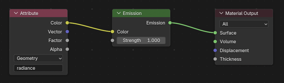
A splat object gets a default material unasked: an Attribute node reading radiance, into
Emission, into the output. radiance returns the splat's colour for the current view
direction: DC plus the higher bands, evaluated against the incoming ray in object space, plus
0.5, converted from sRGB to linear. It is an attribute rather than a node because shape and
opacity are already resolved for that direction in the intersection code.
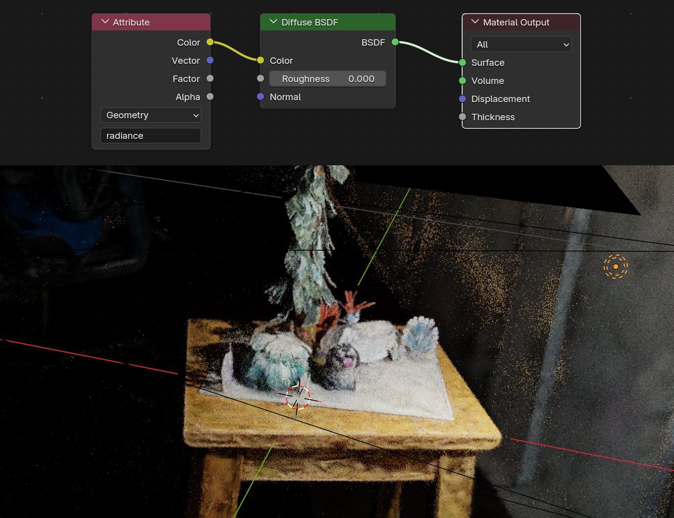
Swap Emission for Diffuse BSDF and the splat responds to Blender's lights through the shortest-axis normal. The notes call this "rudimentary", and rightly: a trained splat's colour already contains the light of the room it was captured in, so lighting it again counts that light twice. The PR names extracting albedo as the future fix.
Limitations: four, not three
Secondary coverage disagrees on how many limitations the release notes list.
Radiance Fields
says three. The primary text has four bullets (reported): performance "is not ideal"; the
splats are assumed to be trained in sRGB; "rendering is not fully correct, as Cycles and EEVEE
operate in linear space"; and Apply Transform does not yet handle scale, rotation or SH. Radiance
Fields folded the second and third into one.
The third is the one to understand. The trainer blends in sRGB; Blender blends in linear light. A 50%-opaque white splat over black blends to 0.5 sRGB (0.214 linear) in one and 0.5 linear (0.735 sRGB) in the other (reasoned from the sRGB curve). The gap is worst where the notes say: low opacity, high radiance, so haze and highlights.
There are more limits in the code than in the notes:
- Speed. The EEVEE PR is plain about it: "The implementation is quite slow. Most existing implementations do tiling/sorting/culling in compute dispatches, which I will work on in subsequent PRs." I have no timing of my own.
- EEVEE's prepass does not work with instancing or multiview yet, and volume light probes
skip splat objects (
eevee_pipeline.cc). - SH degree 4 imports and is then thrown away by every renderer.
- Apply Transform is not just inaccurate. Cycles evaluates SH in object space and asserts that the object transform has not been applied, which is why rotating an object works and baking that rotation into the points does not.
Measured on a real scene
To check the conversions on real data, I read 40 evenly spaced runs of 2,500 splats each,
100,000 in total, from the bonsai scene's point_cloud.ply (iteration 30,000) in the
dylanebert/3dgs dataset on Hugging Face,
at revision 703d19c, using HTTP range requests. The file holds 1,244,819 splats of 62 float32
properties, which is 248 bytes each, after a 1,532-byte header. 1,532 + 1,244,819 × 248 equals
the file's 308,716,644 bytes exactly. I then applied Blender's import formulas from the source
above:
| quantity | value | why it matters in Blender |
|---|---|---|
| SH properties | 45 f_rest, so degree 3 | all of it survives into Cycles and EEVEE |
| opacity below 1/255 | 9.96% | culled by EEVEE and Workbench |
| opacity below 0.01 | 17.37% | radius 0 in Cycles, never hit |
| opacity above 0.99 | 14.35% | effectively opaque discs |
| median opacity | 0.188 | most splats are faint |
| Cycles bound factor | median 2.64σ, max 3.035σ | the sphere is tight for faint splats |
| quaternion length | median 0.9599 (p5 0.784, p95 1.297) | normalization is not optional |
| largest axis ÷ smallest | median 8.23; 44.50% above 10 | most splats are flat, so the shortest-axis normal is well defined |
| largest SH band-1+ magnitude | 0.861 | inside the ±1 that the 8-bit pack keeps |
| DC colour outside 0..1 | 20.74% of splats | the higher bands pull these back; clamping DC early would be wrong |
All measured on the sample; file order is not random, so these are estimates for bonsai, not constants. The inspector's splat is the middle one of 97 that passed a filter I chose for a legible preview (opacity 0.75 to 0.95, anisotropy 3 to 6, a saturated colour): typical-looking, not typical.
Licence
Blender's importer, draw-module and EEVEE code carry SPDX-License-Identifier: GPL-2.0-or-later.
The Cycles kernel files carry Apache-2.0. The SPZ SH-rotation table is credited to Niantic
under MIT, and the glTF importer is Apache-2.0. In practice: your scans and your renders are not
covered by the GPL. If you want to lift the SPZ or PLY importer into a closed-source tool, that
code is GPL and you cannot. If you want the Cycles intersection, it is Apache-2.0 and you can,
with attribution.
What I could not check
- I did not run Blender 5.3. Every behaviour above comes from reading the release branch, not from a render.
- I have no performance numbers. Blender's notes and PRs say it is slow, and nothing more.
- KIRI's clip does not say whether it was rendered in Cycles or EEVEE. The depth-of-field explanation covers both, by different mechanisms.
- The Cycles and EEVEE code cites "Gaussian Point Splatting" (Rijsdijk et al., 2026) for the activation formulas and the 22-bit centre quantization. I did not read that paper.
The capture pipeline in Gaussian-splat capture in practice ends in exactly the PLY Blender now opens; Spirula Studio and KOLC+ edit and place the same data. What Blender adds is a path tracer that treats a splat as something a ray can hit.