2026-10-11 · 24 min · slam · gaussian-splatting · state-estimation · 3d · robotics
Why read this
Nichelast 15%Reads an unreleased GS-SLAM system from its figure and lineage, derives the plane-closure residual, and shows in a toy what one re-seen wall fixes.
- Original analysis
- A lasting reference
- Explained from first principles
Robotics & embodiedNothing to runResearch paper
How this was scored
- Is it new?
- 1 of 3: An incremental tweak
- Can I trust it?
- 1 of 3: Spot-checks a few numbers
- Can I run it?
- 0 of 3: Closed, nothing to run
- Will I understand it?
- 2 of 3: Mechanism from first principles with figures
- Can I act on it?
- 1 of 3: General advice
- Will it last?
- 2 of 3: A reference for a year or more
- Does it affect many?
- 1 of 3: A specialist community
- Only here?
- 2 of 3: A teardown or measurement few others did
Score 45 of 100, ranked 421 of 494 rated articles. Each question is answered 0–3 by hand, and a 3 is rare. How articles are scored
A post by Ryohei Sasaki (@rsasaki0109) on 11 October put StructureGS-SLAM in front of me with four bullet points: persistent Planar Gaussian Instances, "Structure Closure for drift correction without loop revisits", structure-aware Gaussian optimisation, and adaptive RGB-depth consistency for low-texture rooms. The second bullet is the one that made me stop. Loop closure is the only cure for drift that most visual SLAM systems have, and it only works if the robot comes back to somewhere it has been. A robot that drives down a corridor and leaves never gets that chance.
So I went to read the paper and the code, and found neither. The repository the post links,
yanyan-li/StructureGS-SLAM, holds exactly two
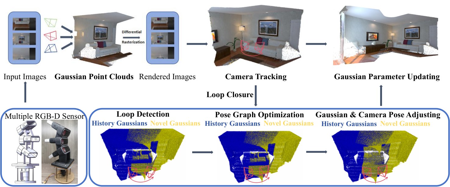
files in one commit (3d35e3d, 1 July 2026): a README and the pipeline figure below. The README
says "The paper will be released soon" and "The source code will be released soon." I searched
the arXiv API by title, by phrase ("Planar Gaussian Instance", "structure closure") and by author,
and the ECVA proceedings page: nothing. The only other trace is Yanyan Li's homepage, which lists
"Structure Gaussian Splatting SLAM" by Y. Li, Y. Li and G. H. Lee as an ECCV 2026 paper and
links its "Project Page" back to the same repository.
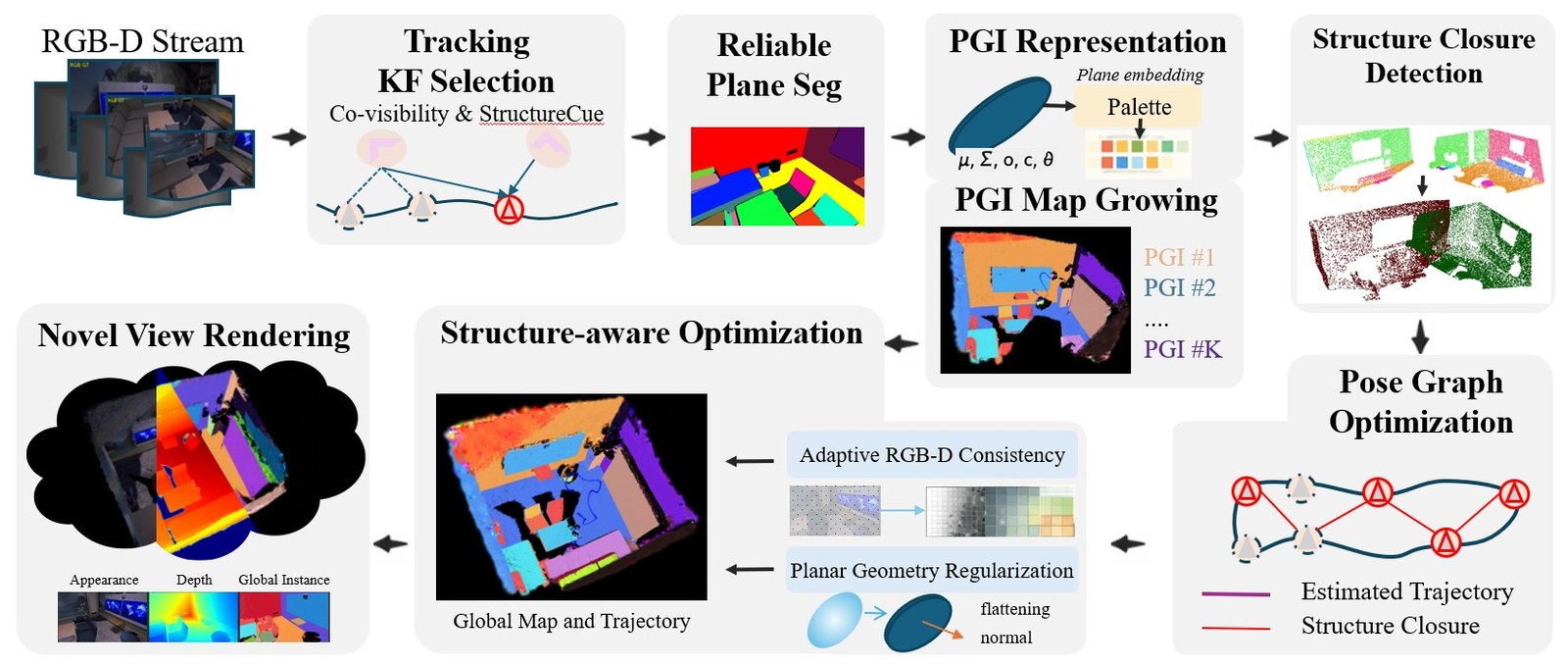
That changes what this article can be. I cannot quote the paper's equations or check its tables, because nobody outside the review process has them. What I can do is read the figure carefully, because it is unusually specific, and read it against the authors' own earlier systems, because the lineage is unusually clear. Yanyan Li has been building plane-based SLAM since 2020 (Structure-SLAM, RGB-D SLAM with Structural Regularities, ManhattanSLAM), wrote a Gaussian splatting method that flattens Gaussians onto surfaces (GeoGaussian, ECCV 2024), and was the corresponding author on a loop-closure module for Gaussian-splatting SLAM. StructureGS-SLAM's figure looks like those three pieces bolted together. Where I describe a mechanism below that the figure does not show, I say it is my reading.
- branch
- main
- tests
- none found
- commit date
- 2026-06-30
local clone, 2026-10-11 at 3d35e3d — branch, commit, commitDate, fileCount, hasTests, shallow
shallow clone: counts describe the pinned tree, not the history
What the repository actually says
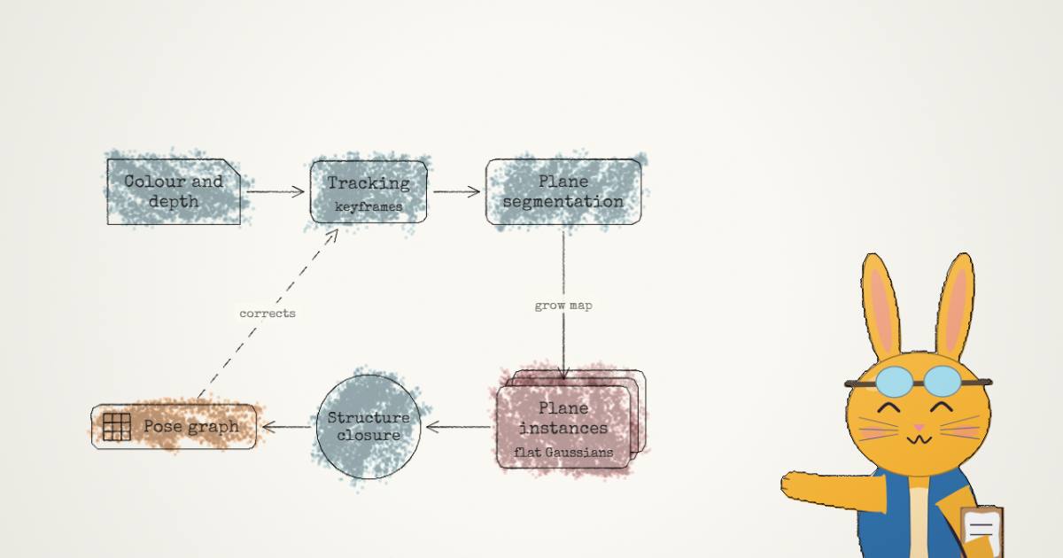
Everything public about the system fits in this figure and fourteen lines of README.
The README's results section claims "state-of-the-art performance on Replica and TUM RGB-D
benchmarks" in pose estimation, novel view synthesis, dense reconstruction and low-texture
robustness. It gives no numbers, names no baselines and does not mention ScanNet. It also says
the project "is released under the MIT License", but the repository has no LICENSE file and
nothing to license yet, which is why the frontmatter above says n/a.
None of that is unusual for an accepted paper waiting on a camera-ready deadline. It just means the four bullets are claims, and the rest of this article is about what each one would have to mean mechanically, and what it would take to believe it.
How a splat map tracks a camera
Gaussian-splatting SLAM swaps the map of a classical system (sparse features, or a TSDF volume) for the thing 3D Gaussian splatting renders: millions of anisotropic Gaussians, each with a mean , a covariance , an opacity and a colour . A camera pose projects each one to a 2-D splat, and front-to-back alpha blending gives a pixel's colour and depth (the capture-pipeline piece covers the offline version, and the colour article what each Gaussian stores):
Because this is differentiable in the pose as well as in the Gaussians, tracking is image alignment against your own map. Freeze the Gaussians, render from a guessed pose, and descend on the residual between the render and the frame that just arrived. The three systems StructureGS-SLAM will be measured against do this differently enough to matter.
SplaTAM (CVPR 2024) uses isotropic Gaussians and a silhouette mask so it only scores pixels the map already explains. The loop-closure paper by Li's group writes its tracking loss in SplaTAM's form, with a fixed half weight on colour:
MonoGS (Gaussian Splatting SLAM, CVPR 2024) derives the analytic Jacobian of the pose, keeps a small covisibility window of keyframes, and in RGB-D mode minimises with for every sequence. It also runs on colour alone, which SplaTAM cannot. Photo-SLAM (CVPR 2024) takes the other road: ORB-SLAM3 does the tracking on sparse features, and the Gaussians are only the photorealistic map hung on those poses.
That last split is the useful one for this article. SplaTAM and MonoGS track against the Gaussians and have no loop closure at all. MonoGS says so in its experiments ("approaches that, like ours, do not have explicit loop closure") and in its limitations: "For larger real-world scenes, the trajectory drift is inevitable." Photo-SLAM inherits ORB-SLAM3's loop closure and corrects keyframes with a similarity transform when it fires.
Why the error never comes back out
Drift in a system like this has a specific shape. Each frame is aligned to a map that was itself built from earlier estimated poses, so any error in those poses is baked into the Gaussians, and the next frame is aligned to the error. Nothing in the tracking loss can see it. A camera that is 2 degrees off in heading renders a map that is consistent with that 2 degrees.
LiDAR odometry has the same disease and the same split of cures; the FAST-LIO2 walkthrough and FAR-LIO are about keeping the increments honest, and SurfSLAM about pulling them back with registrations.
Rotation is the expensive part. A heading error does not stay put; it swings every metre the camera travels afterwards, so position error grows like distance times heading error, and if the heading error itself grows steadily the position error grows with the square of the distance. ManhattanSLAM puts it bluntly: "drift is mostly driven by inaccurate rotation estimations", and the group's 2021 RGB-D SLAM with Structural Regularities cites earlier work showing that "the rotation estimation error is the main reason for long-term drift."
The classical answer has two parts. Loop closure recognises a place it has seen, measures the relative pose between now and then, and spreads the disagreement over a pose graph. Structure-SLAM (2020) states its catch in one sentence: loop closure "removes the drift only when revisiting the same place." The other answer, which Li's group has been working on for six years, is to stop estimating rotation incrementally at all when the scene lets you. In a building, walls, floors and ceilings come in a few directions. If you can see one of those directions, and you remember which way it pointed when you first saw it, you can read your rotation off the wall.
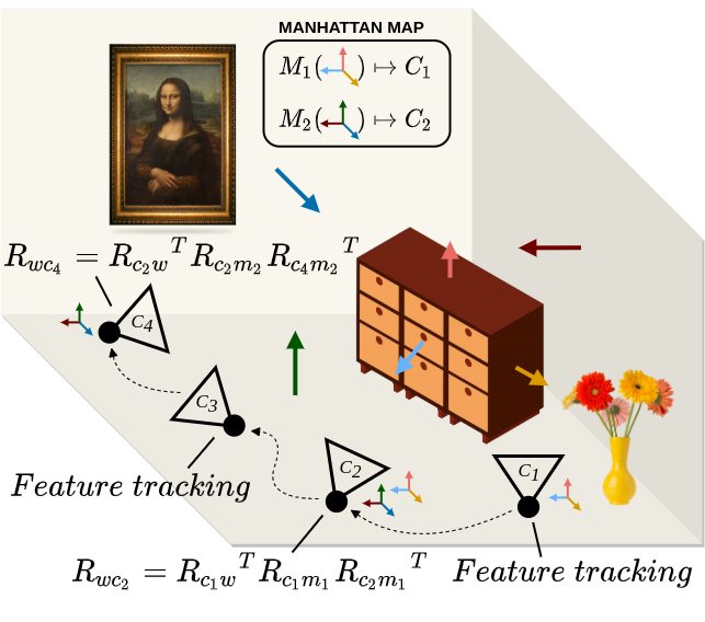
ManhattanSLAM's version of that is exact and cheap. Detect three mutually perpendicular plane normals in the current frame, stack them into a rotation , look up the frame that first saw the same Manhattan frame , and compose:
No chain of frame-to-frame increments sits between and , so no increments' worth of error does either. "Structure Closure ... without loop revisits" is that idea, scaled up from one dominant room frame to every persistent plane in the map, and fed into a pose graph rather than used to overwrite one frame's rotation. At least, that is what the figure draws.
A plane that remembers: the Planar Gaussian Instance
The figure's third and fourth boxes are where the new representation lives. Each Gaussian carries the usual and one more symbol, . An arrow labelled "plane embedding" runs into a "Palette" that maps to a grid of discrete colours, and "PGI Map Growing" shows the room painted in instance colours labelled PGI #1 to PGI #K.
My reading, which the figure supports but does not spell out: is a learned per-Gaussian plane embedding, rendered by the same alpha blending as colour, and the palette assigns each rendered embedding to a plane instance. Instance-aware splatting methods carry identity through a renderer this way, and it is the only reading under which the third render at the bottom of the figure, labelled "Global Instance", makes sense. The word "persistent" then means the instance ID survives across keyframes: plane #3 seen at frame 40 and plane #3 seen at frame 900 are the same object, even if the camera saw it from opposite ends of a corridor.
Where do planes come from in the first place? The box says "Reliable Plane Seg" and shows a segmentation mask, nothing more. In ManhattanSLAM planes come from the depth image through agglomerative hierarchical clustering, downsampled to 0.2 m voxels, and a plane is thrown away if any of its points sits more than 0.04 m off it; that runs on a laptop CPU. Whether StructureGS uses depth clustering, a learned plane segmenter or both, I could not check. "Reliable" suggests a filter of the same kind.
The parameterisation is standard. A plane is a unit normal and an offset, with , and for optimisation ManhattanSLAM uses the minimal three-number form
What makes it a Gaussian instance rather than a sparse plane landmark is the box "Planar Geometry Regularization: flattening, normal". GeoGaussian, by the same first author, did exactly this for offline splatting: in smooth regions each Gaussian is made thin by fixing its third scale to 0.001, the third column of its rotation is the surface normal, and a loss pulls neighbours onto a common plane:
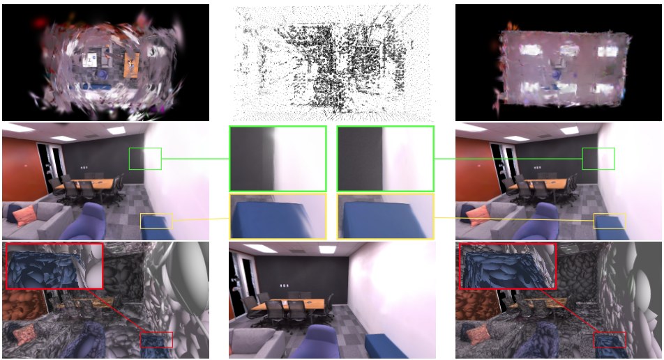
With a PGI the neighbourhood average becomes the instance's own plane, so the regulariser I would expect is a point-to-plane term on every member Gaussian, , a normal-alignment term between the Gaussian's thinnest axis and , and a penalty on that thinnest scale. I am extrapolating from the figure's two words and GeoGaussian's loss, not the paper's equation.
The payoff of doing this inside SLAM, rather than after it, is that the plane is no longer a side product. The Gaussians that render the wall are the wall's plane estimate. When a pose is corrected, the plane moves with its Gaussians, and the next frame tracks against a straighter wall.
Structure closure, written out
Below is the residual I think the "Structure Closure Detection" and "Pose Graph Optimization" boxes compute. The figure gives the boxes and the red edges; the algebra is ManhattanSLAM's plane residual applied between keyframes instead of between a frame and the map.
A world plane seen from a camera with pose appears as
which is in homogeneous form. Suppose keyframes and both observe PGI , and nothing else ties them together: they are far apart in time and may be far apart in space. Map 's observation into through the current relative pose estimate and compare it with what actually saw:
A three-dimensional residual on a six-degree-of-freedom relative pose: it is worth being precise about which three. The two angle components pin the rotation about every axis except the plane's own normal. The offset component pins translation along the normal and says nothing about sliding within the plane. Two non-parallel planes fix rotation completely; three planes with independent normals (two walls and a floor, say) fix all six.
The Manhattan regularity adds edges even between planes that are not the same instance. ManhattanSLAM writes parallel and perpendicular plane constraints as
with a 90 degree rotation and the two angles. Whether StructureGS uses only same-instance closures or also these structural ones, the figure does not say. The panel shows matched plane clouds in two colours, which reads as same-instance matching.
These edges then go into a pose graph next to the ordinary odometry edges (the GTSAM article builds that machinery from first principles). The group's earlier Gaussian-splatting loop-closure paper (Zhu et al., 2024, Li as corresponding author) gives the form, minimising over keyframe rotations and translations :
A structure closure is just a different kind of edge in , one whose measurement comes from a shared plane rather than from a recognised place, and which constrains only three of the six directions.
The piece that makes this practical for a splat map is the step after the solve. In that loop closure paper every Gaussian remembers the keyframe that spawned it, and when that keyframe's pose changes from to its Gaussians move rigidly with it:
The paper says the covariance "does not need to be updated". That holds there because its Gaussians are isotropic (all three scales are set equal), so rotating one changes nothing. Flattened planar Gaussians are the opposite case: rotate the anchor and each thin Gaussian's orientation has to turn with it, or the wall's normals stop agreeing with the wall. Either way, the map follows the trajectory without re-optimising millions of Gaussians from scratch, and the "structure-aware optimisation" box then cleans up what the rigid move leaves behind.
The whole idea fits in a toy. A robot drives about 60 m around the inner block of a rectangular floor (east, north, west) and stops 14 m north of where it began. It never revisits anything. Odometry has a constant yaw bias. The west wall is one persistent plane: seen in the first couple of metres, out of view for most of the run, and seen again at the end from a different place.
- end error, odometry
- 7.98 m
- end error, corrected
- 0.30 m
- ATE RMSE odo / corr
- 3.52 / 0.17 m
- heading error at end
- 31.0° / 1.0°
About 58 m in, the robot sees the west wall again from 14 m north of where it first saw it. The stored plane and the re-observed one disagree by 30.0° in normal and 0.06 m in offset. The heading residual is spread linearly over every pose since the start, the path is re-integrated, then the offset is spread the same way along the wall's normal. One plane fixes heading and the east-west position; the north-south error it cannot see is what is left. Toy model: all noise levels, ranges and gates are mine, not the paper's.
At the default 0.50 degrees of drift per metre, dead reckoning ends 7.98 m from the truth with a heading 31.0 degrees off, and an absolute trajectory error (ATE RMSE) of 3.52 m. About 58 m in, the west wall comes back into view, and the stored plane and the re-observed one disagree by 30.0 degrees in normal and 0.06 m in offset. Spread that rotation linearly over every pose since the start (the exact least-squares answer for a rotation chain with equal weights, and the same trick SurfSLAM's drift toy uses for translation), re-integrate, then spread the offset along the wall's normal, and the run ends 0.30 m from the truth with an ATE of 0.17 m. Look at what is left: almost all of it is north-south, along the wall. One plane fixed heading and the east-west position and could not see the third direction, exactly as the algebra above says.
Switch on the Manhattan frame and every visible wall pins the heading on every step; the end error drops to 0.09 m. Then tilt the north wall by 6 degrees. The Manhattan snap still forces it onto the nearest axis, and on the last leg the heading is dragged about 3 degrees the wrong way (half the tilt, because the straight wall across the corridor votes the other way). The run now ends 0.84 m out, worse than the plain plane closure. And at zero drift the plane closure makes things slightly worse (0.33 m against 0.17 m at the end), because it is fitting a straight ramp to what is now only noise. Every noise level, range and gate in the toy is mine.
Low texture: weighting colour against depth
The fourth bullet, "adaptive RGB-depth consistency", has one small panel in the figure: an image patch with a sparse sprinkling of dots, an arrow, and a grid of grey and coloured tiles. That is too little to reconstruct a formula from, so here is the problem it addresses and the obvious design.
Every baseline above weights colour and depth with a global constant: SplaTAM's form gives colour half the weight of depth, MonoGS uses on every RGB-D sequence. On a white wall the photometric residual is flat in the pose directions that slide along the wall, so its gradient is noise; on a bookshelf it is the best signal you have, and depth there is ragged at every edge. A per-region weight fixes the mismatch:
with rising with local image gradient (or with the number of trackable points in a tile, which is what the dotted patch in the figure hints at). This is my sketch, not the paper's loss. It is also not a new idea in kind: MonoGS already notes that it "penalise[s] non-edge or low-opacity pixels" in its photometric term. What might be new is doing it per tile and letting the planar Gaussians carry the depth term where colour gives up. A white corridor is where a plane prior earns its keep twice: it is the scene where photometric tracking is weakest and the scene with the largest planes.
The numbers it will be judged against
The README claims state of the art on Replica and TUM RGB-D. The bar looks like this, from each baseline's own paper. ATE is RMSE in centimetres; PSNR is on Replica, rendered mostly at the views the system tracked, which is how these papers report it.
| System | Input | Replica ATE | TUM ATE | Replica PSNR | Speed reported |
|---|---|---|---|---|---|
| SplaTAM | RGB-D | 0.36 | 5.48 (5 seqs) | 34.11 | 1.00 s tracking + 1.44 s mapping per frame, RTX 3080 Ti |
| MonoGS | RGB-D | 0.58 (0.32 single-process) | 1.47 (3 seqs) | 38.94 | 2.5 FPS on fr3/office, RTX 4090 |
| MonoGS | RGB only | n/a | 3.96 (3 seqs) | n/a | 3.2 FPS on fr3/office |
| Photo-SLAM | RGB-D | 0.604 | 2.603 / 0.346 / 1.001 | 34.958 | 42.485 tracking FPS, RTX 4090 |
| Photo-SLAM | RGB only | 1.091 | 1.539 / 0.984 / 1.257 | 33.302 | 41.646 tracking FPS |
| ORB-SLAM2 | RGB-D | n/a | 1.98 (5 seqs) | n/a | (SplaTAM's table) |
Photo-SLAM's TUM numbers are fr1/desk, fr2/xyz and fr3/office. MonoGS's three sequences are the same; SplaTAM's five add fr1/desk2 and fr1/room, which is why its 5.48 cannot be set next to MonoGS's 1.47 as if they measured the same thing. On SplaTAM's own five sequences, ORB-SLAM2, a sparse-feature system from 2017, beats it, 1.98 to 5.48.
Two things in this table shape how I will read StructureGS-SLAM's results when they appear.
Replica is close to saturated for tracking. Three systems sit within a quarter of a centimetre of each other, on synthetic rooms with perfect depth and, in SplaTAM's words, "small displacements between consecutive camera poses." A structure closure has very little drift to remove there, and a win of a tenth of a millimetre would tell me nothing about drift. TUM is the test that matters: real Kinect depth with holes, motion blur, and in fr1/room a trajectory long enough to drift. The sequence choice will matter as much as the method (the Hilti datasets article is a long argument about how much the scoring choice moves a ranking); three easy TUM sequences and five mixed ones give different pictures, as the table shows.
The phrase "without loop revisits" also needs a sequence that has none. Most standard TUM and Replica trajectories wander around one room and see every wall many times, so closure-by-revisit and closure-by-structure are hard to tell apart on them. The experiment I would want is an ablation on a corridor or multi-room sequence where a classical loop detector provably never fires, with ATE with and without structure closure. If the paper has that, the claim is tested. If it only reports Replica and three TUM rooms, it is not.
Runtime is the other unknown. Plane segmentation, a rendered embedding channel and a pose graph are each cheap next to Gaussian optimisation, but SplaTAM and MonoGS already run at one to three frames a second. Photo-SLAM's 42.485 FPS comes from sparse-feature tracking; a system that tracks by rendering will not get near it. Whether StructureGS tracks by rendering, by features, or by planes directly, the figure does not show; the first box only says "Tracking".
ScanNet is not in the README at all. For reference SplaTAM averages 11.88 cm ATE on its six ScanNet scenes, the noisiest of the standard benchmarks. A plane method should do well there (lots of walls, bad colour), so its absence from the claims is something I will look for in the paper.
Where planes lie
The planar prior is a bet on the scene. I think it loses in four places, ordered from the most to the least likely to bite in practice.
Corridors give you fewer constraints than they seem to. Two parallel walls and a floor have only two distinct normal directions between them, so translation along the corridor is unobservable from structure alone, the same failure the toy shows with one wall. A corridor is also where photometric tracking is weakest. Structure closure fixes the heading in a long corridor, which is most of the drift, and leaves the along-track error to odometry.
Not every wall is square. Under a Manhattan assumption a wall 6 degrees off axis is not ignored, it is believed, and the toy shows the cost: a confidently wrong constraint is worse than none. ManhattanSLAM's whole contribution over its predecessors was noticing this, modelling the scene as a mixture of Manhattan frames and falling back to feature tracking when no frame is detected. If StructureGS-SLAM's closures are same-instance only, it is safe from this; if they include structural parallel and perpendicular edges, it needs the same fallback.
Association is the real risk. Two parallel walls in a symmetric corridor, or two identical doors, have the same normal and similar offsets. A wrong plane match in a pose graph is a wrong loop closure, and those are the classical way to wreck a map. The figure's "Reliable Plane Seg" and "Structure Closure Detection" boxes are where that is handled, and they are the boxes I most want to read the paper for.
Clutter and outdoor scenes shrink the prior. GeoGaussian's own limitations section says "The geometric constraints degenerate if few smooth regions are detected" and "Incorrect geometric residuals can occur when fake smooth regions are initialized as thin Gaussians." Outdoors there is usually one reliable plane (the ground), RGB-D depth gives out at a few metres, and building facades are far away. A sofa or a curtain that segments as a plane becomes a wrong instance. One reply under the post made the case that closure without revisits matters most in the air, where a survey flight never crosses its own path; I agree with the motivation and doubt the transfer, because from altitude the only large plane is the ground.
There is prior art inside Gaussian splatting too. MG-SLAM (Liu et al., 2024) is "Structure Gaussian Splatting SLAM with Manhattan World Hypothesis", from a different group, and used line features for tracking in textureless rooms and Manhattan planar surfaces to fill holes in floors and ceilings. What StructureGS-SLAM's figure adds over it is persistence (plane instances with identity) and the closure edges in a pose graph. Whether that is a large step depends on numbers I cannot see yet.
What I make of it
The idea is good and old in the best way. Using the building as a compass is how structure-based visual SLAM got low drift without loop closure years ago, and Gaussian splatting is a natural host for it: the map is already made of small oriented primitives, and flattening them onto a plane both improves the render on textureless walls and turns the wall into a measurable landmark. The rigid re-anchoring trick from the same group's loop-closure paper is what lets a pose-graph correction reach the Gaussians cheaply. Put together, the four bullets are coherent.
What I would not do yet is repeat the claim. "Drift correction without loop revisits" is true of rotation and of translation along plane normals, and only when the planes are real, square or matched correctly, which the toy above makes concrete. The README's claim of state of the art on Replica and TUM has no table behind it in public. When the paper lands, the things I will check first are the TUM sequence list, whether there is a no-revisit sequence with a closure ablation, the runtime and its hardware, and how plane association is gated. I will update this page then.
How I checked
- Cloned
yanyan-li/StructureGS-SLAMwithgit clone --depth 1on 11 October 2026: one commit (3d35e3d, 2026-07-01), filesREADME.mdandasset/architecture.jpg. The README text quoted above is lines 9-36. The X post's image is the same figure (1,654 by 701 pixels). - Searched the arXiv API by exact title, by the phrases "Planar Gaussian Instance", "structure closure" and "StructureCue", and by author; searched the ECVA proceedings page for ECCV 2026. No paper is public. The ECCV 2026 acceptance and author list are from Yanyan Li's homepage.
- Read, in full, ManhattanSLAM (arXiv 2103.15068), RGB-D SLAM with Structural Regularities (2010.07997), Structure-SLAM (2008.01963), GeoGaussian (2403.11324), the Gaussian-splatting loop-closure paper (2409.20111), MG-SLAM (2405.20031), SplaTAM (2312.02126), MonoGS (2312.06741) and Photo-SLAM (2311.16728). Every baseline number in the table is copied from the named paper's own table, with its sequence set and hardware.
- The plane-closure residual and the adaptive weighting formula are my derivations from the figure and the prior papers. They are labelled as such where they appear.
- The toy (
components/articles/structuregs-slam/sim.ts) is a 2-D simulation with seeded noise: 0.25 m steps, 2% step-length noise, 0.05 degrees of heading noise per step, walls seen within 4.5 m, a closure needing 10 m of travel out of view. None of it is StructureGS-SLAM's code, because none has been released.