2026-10-06 · 25 min · 3d · gaussian-splatting · cuda · benchmarks
Why read this
Notabletop 60%Each 3DGS colour model's maths and CUDA, bytes recounted from code, the M360 table split (SH still wins outdoors), and what it means for a capture pipeline.
- Original analysis
- Runs on a consumer GPU
- A lasting reference
3D & spatialApache-2.0Practitioner paper
How this was scored
- Is it new?
- 1 of 3: An incremental tweak
- Can I trust it?
- 2 of 3: Measures key facts from files, code or configs
- Can I run it?
- 2 of 3: Open code or weights with real limits
- Will I understand it?
- 2 of 3: Mechanism from first principles with figures
- Can I act on it?
- 2 of 3: A concrete recipe, numbers or comparison
- Will it last?
- 2 of 3: A reference for a year or more
- Does it affect many?
- 1 of 3: A specialist community
- Only here?
- 2 of 3: A teardown or measurement few others did
Score 62 of 100, ranked 211 of 445 rated articles. Each question is answered 0–3 by hand, and a 3 is rare. How articles are scored
When I wrote up how people capture Gaussian-splat scenes with 360 cameras, one number kept coming back. A 15-million-splat drone capture of a dam was trained at spherical-harmonic degree 2, and when someone asked why not degree 3, the answer was two words: "VRAM limitation". The arithmetic behind that is not subtle. At degree 3, 48 of a splat's 59 trainable floats are colour, and 45 of those exist only to make the colour change with viewing direction.
So when Florian Hahlbohm posted "It's time to stop defaulting to spherical harmonics for 3DGS!", I read the whole ten-post thread, the paper and every CUDA function in the code. The pitch is a compact neural appearance model: 28 bytes per Gaussian instead of 192, faster training, a little better PSNR on average. The work is bigger than the pitch. They took five appearance models (SH, Spherical Voronoi, NASG, NASGabor and theirs), put all of them into one optimised pipeline with the same densification and the same everything else, and measured quality, memory, training time and frame time on desktop GPUs and a phone.
Three things surprised me. The neural model still uses spherical harmonics; it just stops storing them per Gaussian. On the outdoor scenes of Mip-NeRF 360, plain SH still has the best PSNR of the lot. And the most useful part of the paper is not a model at all. It is an argument about what the "view-dependent" part of a splat actually learns on a real capture, and it should change how anyone running a capture pipeline reads benchmark tables.

The colour of one Gaussian, as a function of direction
A Gaussian splat has a position, a shape, an opacity and a colour. The colour is not one RGB triple, because real surfaces look different from different angles: a varnished table, a laptop lid, wet stone. So 3DGS makes colour a function of the unit direction from the camera to the Gaussian's centre. The paper writes every model in the same form, which is what makes the comparison fair:
is a view-independent base colour, is the view-dependent residual (the thing being compared), and is a colour activation. Standard 3DGS uses . Only changes between models. Base colour, its initialisation from the SfM point colours, its densification handling: all identical.
Spherical harmonics
For SH, the residual is a weighted sum of fixed basis functions on the sphere, with one RGB weight per function:
Degree contributes functions, so degrees 1 to 3 give functions, times three
colour channels: 45 numbers. Add the base colour and you have the 48 fp32 values, 192 bytes, that dominate
a 3DGS file. The basis functions are polynomials in the components of of degree at most 3. In
the CUDA that is all there is, a straight-line expression over (appearance_sh.cuh:43-61):
// FasterGSVDACudaBackend/.../rasterization/rtc/appearance_sh.cuh
float3 result = -sh_c1 * y * coefficients_ptr[0]
              + sh_c1 * z * coefficients_ptr[1]
              - sh_c1 * x * coefficients_ptr[2];
// ... degree 2: five more terms in xy, yz, zz, xz, xx - yy ...
// ... degree 3: seven more terms, cubic in x, y, z ...
return residual_activation(result);
That explains both of SH's habits. It is cheap and trains easily: everything is linear in the coefficients, and 3DGS switches one degree on every 1,000 iterations so view dependence comes in late. It is also band-limited. A cubic polynomial on the sphere cannot make a highlight that is bright over a few degrees and dark elsewhere; it can only make a broad bump with ripples around it. The paper's other complaint is about cost: SH coefficients "dominate per-primitive storage and memory traffic", and Adam has to update all 45 of them for every Gaussian every step, including ones not visible in that iteration's image. The paper cites its own earlier Faster-GS measurement that SH updates alone can take up to 50% of optimisation time at high primitive counts.
Spherical Voronoi: a soft partition of the sphere
Spherical Voronoi (SV) places sites on the sphere, each with a colour and a temperature , and blends the site colours by a softmax over distance to the view direction:
With high temperatures this is a hard Voronoi partition: look from inside one cell and you see that
site's colour. It can make sharp angular edges SH cannot. Two details matter. The softmax weights sum to
one, so a single site gives a constant and you need at least two for any view dependence. And each site
costs 7 floats (direction, temperature, RGB), so the default seven sites are 49 floats plus the base
colour: 208 bytes, more than SH. The implementation here improves on the reference by computing the
softmax in one pass with a running maximum (appearance_sv.cuh:41-56), reading each site once instead of
three times.
NASG and NASGabor: one sharp, stretched lobe
Normalized anisotropic spherical Gaussians come from Miazga et al.,
who adapted them from neural path guiding. A lobe has a frame (axis , tangent ),
a sharpness and an anisotropy . With and
, the code's own header comment (appearance_nasg.cuh:6-14) spells it out:
Read it slowly and it is a spherical Gaussian , peaked on the axis, whose width is squeezed along by the factor when . normalises it so sharpening a lobe does not change how much colour it contributes overall. The bounds each lobe's contribution so the residual cannot run away from the base colour. A lobe is 8 numbers: three frame angles (stored as cosines through a ), , and RGB. The paper uses one lobe, the reference default: bytes.
NASGabor multiplies the lobe by a non-negative cosine carrier along the tangent,
, with , so between 0 and 40
(appearance_nasgabor.cuh:13). One extra number buys a lobe that can have several bright bands, a cheap
way to get a multimodal reflection from one kernel. 48 bytes.
The whole difference between SH and a lobe is easier to see than to read. The widget below takes one Gaussian and looks at it from every direction around a circle. On a great circle, real SH up to degree span exactly the Fourier modes up to order , so the least-squares SH fit is a truncated Fourier series; the lobe fit is a 1D cut of a spherical-Gaussian lobe, fitted by exhaustive search. Slide the sharpness up.
Target: a diffuse colour plus one reflection that sharpens as the slider rises.
At the default sharpness (, a highlight roughly 30 degrees wide), degree-3 SH reaches a peak of 0.63 where the target is 0.85, and smears the rest of that highlight around the circle; one lobe fits it to within the search grid. Push to the right and SH gets worse while the lobe barely notices, which is the point of NASG. On the full sphere degree-3 SH stores 16 functions per colour channel, of which this circle exercises only 7; the bytes bar counts all 16. Then try the third target, which has no reflection in it at all. Hold that thought.
The neural model: per-Gaussian codes, one shared decoder
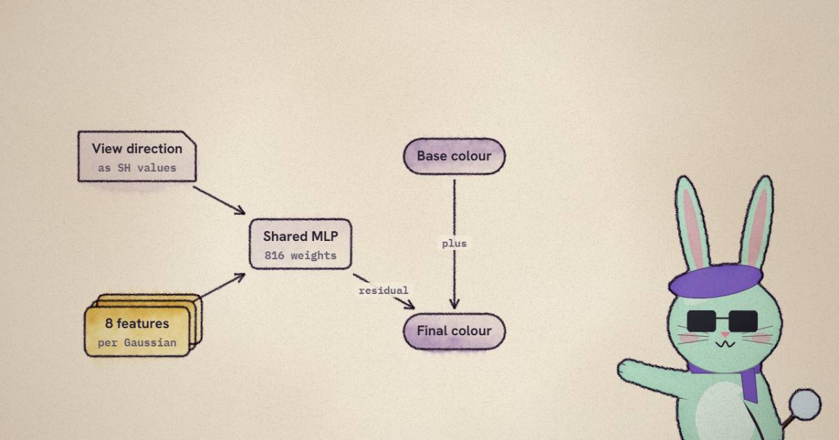
The paper's own model drops the idea of a per-Gaussian basis expansion. Each Gaussian stores a feature vector , and one small MLP, shared by every Gaussian in the scene, maps features plus view direction to a residual:
The feature encoding is a one-frequency sinusoid per feature, ,
so 8 features become 16 inputs. The direction encoding is the part I did not expect:
is the SH basis of degrees 0 to 3, evaluated at , which is
more inputs. The kernel literally calls eval_sh_degrees(direction, ...) to fill the
second half of the MLP input (appearance_neural.cuh:332). Spherical harmonics have not gone anywhere.
What is gone is the 45 per-Gaussian weights. The basis values are computed on the fly and cost nothing to
store, and the weighting is done by a network that is shared, so the per-Gaussian part shrinks to an
8-number code that tells the shared network which kind of surface this is.
The sizes are chosen by the hardware. Tensor Cores want the input width to be a multiple of 16; the
degree-3 direction encoding is already 16, so 32 is the smallest width that leaves room for features, and
16 inputs fit 8 features at one frequency. Neural.py:35 warns if the width is anything but 32. The
network is 32 to 16 to 16 to 3, ReLU, no biases (the constant degree-0 SH input does the job of one), so
the whole scene's decoder is weights. The output layer starts at
zero (Neural.py:53) and so do the features, so the residual is exactly zero until training gives it
something to say, and the direction bands switch on one per 1,000 iterations on the same schedule as SH.
The footprint arithmetic is worth doing yourself, because the paper's 28 is a deployed number:
| model | per-Gaussian appearance | bytes |
|---|---|---|
| none (base colour only) | 3 fp32 | 12 |
| SH degree 3 | 48 fp32 | 192 |
| Spherical Voronoi, 7 sites | 3 + 7 × 7 fp32 | 208 |
| NASG, 1 lobe | 3 + 8 fp32 | 44 |
| NASGabor, 1 lobe | 3 + 9 fp32 | 48 |
| neural | 3 fp32 + 8 fp16 | 28 |
Every row matches Table 1. The neural row assumes the features are stored in fp16, which the paper
justifies: the fused forward and backward run in half precision, so deploying in 16 bits loses nothing.
During training, though, the features are an fp32 tensor (Neural.py:70), so the training-time footprint
is 44 bytes, the same as one NASG lobe. That matters for the memory budget later.
Why it is fast: the decoder lives inside the rasterizer
A per-Gaussian MLP sounds expensive, and the paper says that belief is why nobody did this. The fix is fusion. 3DGS renders in two kernels: a per-primitive preprocess that projects each Gaussian, counts the tiles it touches and computes its colour, then a per-tile blend. Every appearance model here is evaluated inside the preprocess kernel, only for Gaussians that survived culling, with no separate launch and no round trip through global memory.
For the neural model this uses tiny-cuda-nn's fully fused MLP,
which runs one warp per 32 Gaussians on Tensor Cores in fp16. That has a consequence you can see in the
kernel. A Tensor Core matrix multiply needs every lane of the warp, so the network has to run before any
thread is allowed to exit, even for Gaussians that will turn out to touch no tiles
(preprocess_forward.cu:202-216):
#if JIT_APPEARANCE_MODEL == 5
    // residual mlp evaluation where all lanes of surviving warps must participate (warp-cooperative mma)
    tvec<__half, 3> mlp_output;
    const float3 residual = neural_residual(appearance, mean3d, cam_position[0],
                                            fwd_ctx, mlp_output, primitive_idx, appearance_degree);
#endif
    // cooperative threads no longer needed
    if (n_touched_tiles == 0 || !active) return;
Warps that are culled entirely zero their slice of the saved activations before leaving, because the
backward pass runs the MLP backward for every thread and "0 x garbage may be NaN" (the comment on
zero_warp_fwd_ctx). Weight gradients accumulate in fp16 with a loss scale of 128, a power of two, so
undoing it is an exponent shift with no rounding.
How much fusion buys is in the paper's ablation (Table 8): the same model through the unfused reference path trains in 16m08s instead of 4m17s and renders at 112.1 FPS instead of 443.6, with the same quality. A neural appearance model that runs as a separate PyTorch pass is a different, much slower object.
The plumbing is a small piece of good engineering. Each model is one CUDA chunk with a *_residual and a
*_residual_backward device function. At first use, assemble_rtc_source (appearance.cu:78-140) writes
a preamble of #define JIT_APPEARANCE_MODEL, the number of lobes or sites, the activations and the MLP
widths, pastes the chosen chunk and the tiny-cuda-nn device functions in front of the preprocess kernel,
and compiles the lot with NVRTC. Because every configuration value is a compile-time constant, the
specialised kernel has no branches on model type. Adding a model is one Python class and one CUDA chunk,
which is what the thread advertises. Along the way a tiny-cuda-nn bug turned up (the acknowledgements
credit Jannis Möller with finding it): its JIT backward pass evaluated hidden-activation derivatives on post-activation values, instead of .
It is harmless for ReLU, whose derivative depends only on sign, and wrong for every smooth activation.
setup.py:86-110 patches the vendored header at install time, with the reasoning in a comment.
- license
- Apache-2.0
- branch
- main
- tests
- none found
- source
- 673.9 kB
- commit date
- 2026-09-30
by size of tracked source at this commit, file counts in brackets; docs, data and vendored trees excluded
Read at 4efbe67 (30 September 2026). Apache-2.0. The five appearance models are rasterization/rtc/appearance_*.cuh (forward and backward each) plus Appearance/*.py; the JIT assembly is rasterization/src/appearance.cu; the WebGL viewer is viewer/. Needs an NVIDIA GPU with compute capability 7.5+ and CUDA 11.8+ for the fused kernels, and installs into the NeRFICG framework.
local clone, 2026-10-07 at 4efbe67 — branch, commit, commitDate, fileCount, hasTests, languages, license, licenseFile, shallow
shallow clone: counts describe the pinned tree, not the history
What the tables say, and what the average hides
The comparison is controlled in the way that matters: MCMC densification with the same scene-specific primitive budgets for every model, the same 30k iterations, PPISP on real scenes so per-image exposure drift is not learned as view dependence, and five training runs averaged for image metrics. Timings and memory are from the first run on an RTX 4090.
On Mip-NeRF 360 the PSNR order is SV 28.64, neural 28.55, NASGabor 28.54, NASG 28.50, SH 28.36, and no view dependence at all 27.73. SSIM goes the other way for the neural model: SH, NASG and NASGabor share 0.836 and the neural model is last of the view-dependent ones at 0.831. The paper says as much, and its summary table calls the neural model "hard to regularize per scene". On Tanks and Temples plus Deep Blending the neural model has the best PSNR (28.13 against 27.96), and on NeRF Synthetic it matches SH (34.04 against 34.01) while the lobe models fall behind with one lobe each.
The cost side is clearer than the quality side. On Mip-NeRF 360, SH trains in 6m12s, NASG in 3m54s, NASGabor in 4m00s and the neural model in 4m17s; peak memory falls from 6.7 GiB to between 4.9 and 5.3. The "1.3× faster" in the abstract is the conservative end: 6m12s over 4m17s is about 1.45×, and the smallest of the three dataset ratios, NeRF Synthetic's 1m22s over 1m02s, is about 1.32×. The lobe models train faster still. SV, despite its quality, is slower than SH and the largest of the lot.
Rendering tells the same story. In CUDA on the RTX 4090 (Table 2, 720p), NASG and NASGabor are the fastest: 2.25 ms against SH's 2.75 ms on the 6M-Gaussian bicycle, the "up to 18% faster" in the text. The neural model is third. In the WebGL viewer, which has no Tensor Cores, the differences mostly vanish: on an iPhone with an A18 Pro the bicycle takes 45.0 ms with SH and 45.1 ms with the neural model, and SV runs out of memory on the two largest scenes.
Outdoor and indoor are different stories
The Mip-NeRF 360 average mixes five outdoor scenes and four indoor ones. Appendix Table 9 gives every scene, so I split them. The view-dependent models against SH, mean PSNR:
| model | outdoor (5 scenes) | indoor (4 scenes) |
|---|---|---|
| none | 25.05 (−0.44) | 31.08 (−0.87) |
| SH | 25.49 | 31.95 |
| SV | 25.38 (−0.10) | 32.71 (+0.77) |
| NASG | 25.38 (−0.11) | 32.40 (+0.46) |
| NASGabor | 25.40 (−0.09) | 32.47 (+0.52) |
| neural | 25.33 (−0.15) | 32.56 (+0.61) |
Outdoors, SH beats every alternative, and turning view dependence off entirely costs less than half a dB. Indoors, every alternative clears SH, by 0.46 to 0.77 dB. The "matches or exceeds SH in PSNR on average" headline is an average of a loss and a win. The authors do say this, in the appendix: outdoor scenes are "dominated by diffuse content and their remaining error is largely geometric", while indoor scenes have glossy surfaces under controlled lighting. It deserves to be in the abstract, because whether you should switch depends almost entirely on which of those two you capture.
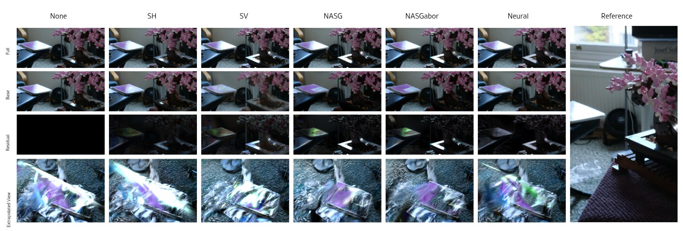
The geometry effect is the most convincing evidence that the expressive models are doing something real. Figure 2 shows the bonsai scene's sketch block. With SH, the reflection on the block is faked by elongated white Gaussians, which in an extrapolated view become streaks; with NASG or NASGabor the reflection sits in the residual and the base colour is a clean diffuse block. This is the same failure I described in the reconstruction roundup: when the colour model cannot make a spike, the optimiser makes matter instead.
One more number belongs here. With a tenth of the primitive budget (Table 7), SH, NASGabor and the neural model land at 27.30, 27.32 and 27.30 dB. When geometry is the bottleneck, no amount of angular expressivity helps.
Footsteps in the grass
This is the part of the thread I would have put first. Posts 6 to 8 are about content that changed during capture. In the Mip-NeRF 360 garden scene, the camera operator stepped on the grass around the table. Rendered top-down with SH, the residual shows a ring exactly where the footsteps went.
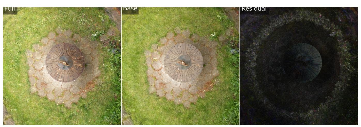
The mechanism is simple once you see it. A capture is a trajectory, so viewing direction and time are correlated. If the grass was upright when the camera was on the north side and flattened by the time it reached the south, then "colour depends on direction" explains the photos perfectly well. The third target in the widget above is exactly this: no reflection, just a change halfway round. Degree-3 SH fits it fine, because a smooth step is low-frequency. An expressive model fits it too, and in the bonsai scene, where a book moved between shots, NASGabor fits it better than SH can.
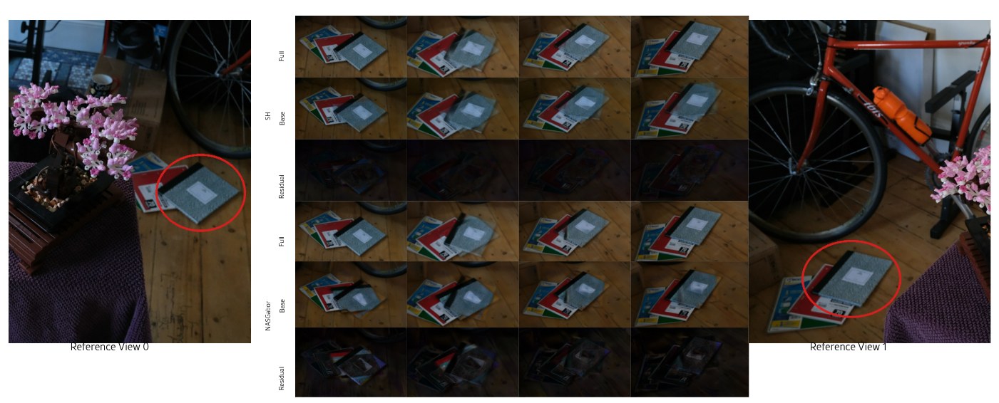
The paper's conclusion is careful and I agree with it: on real benchmarks, part of the advantage of an expressive model may be "robustness to violations of the static-scene assumption" rather than better modelling of outgoing light. Better PSNR on held-out views of an inconsistent scene does not mean a more faithful scene. Synthetic benchmarks avoid the problem but bring their own bias, because they are mostly diffuse hard surfaces. Thread post 8 asks the open question plainly: should we reconstruct one specific state, a motion-blurred version, or a dynamic model? None of the three is easy from current data, and the authors say they do not have the answer.
I think there are two practical readings. If you render for people, an expressive residual that soaks up
a passing shadow is often what you want; it keeps the geometry clean, and the thread and project page point out that
methods that cannot hide errors by popping (sorted-per-pixel renderers like HTGS,
opaque-surface representations like MeshSplatting) should benefit most.
If you measure from the splats, as in a BIM or earthwork workflow, the residual
is also a free diagnostic. Render it on its own, the way Figure 5 does, and it shows you where the scene
changed under the camera. This repository's configs expose it directly as RENDER_BASE_COLOR and
RENDER_RESIDUAL_COLOR.
Where it breaks
The authors list the limits themselves, and two of them matter in practice. None of these models can do a mirror; that still needs secondary rays. And the neural decoder cannot be rotated analytically the way an SH expansion can, so moving or composing objects needs the inverse transform applied to the view direction before the network sees it. A single shared decoder may also run out of capacity on a large scene; the paper suggests a grid of decoders interpolated by camera position, as in SMERF. I would add that it does not always decompose cleanly. On the Dr Johnson scene (Figure 6) the neural model puts the desk's highlight into the base colour, so the "diffuse" render still has a highlight baked in.
The architecture ablation (Table 8) is reassuring about the decoder itself. One hidden layer, three, or 32 neurons all land within about a quarter of a dB of each other, and the differences sit in the indoor scenes. Doubling the per-Gaussian code to 16 raw features is the only variant that costs storage (44 bytes), and it does no better than a deeper decoder. Capacity in the shared network is free; capacity per Gaussian is paid by every Gaussian. That asymmetry is the whole design.
What I would change in a 360-camera capture pipeline
The site owner's own pipeline is a 360 camera, Spirula Studio or LichtFeld for SfM and training, and a web viewer at the end, often through SOG. This is how I would use the paper there.
Training memory is where the alternatives pay off. Using the same naive count as before (four fp32 copies of every trainable float: value, gradient and two Adam moments), a Gaussian here has 11 geometry floats plus its appearance: 59 floats at SH3, 38 at SH2, and 22 for one NASG lobe or the neural model in training precision. At 15M splats that is 14.16 GB, 9.12 GB and 5.28 GB of optimiser state, before images and scratch buffers. A single-lobe model costs less than the SH2 run that the dam capture had to settle for, and keeps sharper highlights than SH3. The measured peaks in Table 1 move the same way, 6.7 GiB for SH against 4.9 for NASG on Mip-NeRF 360.
Delivery is where SH still wins. The paper mentions it in passing; the author spelled it out in a reply. The SOG format vector-quantizes the 45 SH-rest values of every splat into a shared palette of up to 65,536 entries and stores one 2-byte index per splat. The paper's own WebGL viewer packs SH into 40 bytes with Spark's bit-packed layout, against 32 bytes for the neural payload. When someone asked Hahlbohm what blocks mainstream adoption, his answer was the lack of NPU access from WebGL and WebGPU for the neural model, and, for the lobe models, "how much more explored compression/quantization of SH-based 3DGS is". The paper itself stores the lobe models in plain fp16 in its viewer and leaves comparable quantization schemes for them to future work.
The export path makes the same point harder. convert_to_ply for any non-SH model writes only the base
colour, with a warning that the view-dependent residual is not included (Base.py:230-236). A NASG or
neural splat loaded into a standard viewer is a diffuse splat. If you train with one of these models
today, you either ship through this repository's viewer, which uses its own .ngsplat format, or you
accept losing the view dependence at the boundary.
So my rule of thumb from these numbers:
- Outdoor drone or walking captures, mostly diffuse: Keep SH, and drop to degree 1 or 2 if memory is tight. Outdoors the alternatives do not beat SH on PSNR, and no view dependence at all trails SH by about 0.44 dB on average.
- Indoor, glossy surfaces, controlled light: Train a lobe model (NASG is the simplest, and the paper's summary table says the "Gabor term is not worth it outside standard benchmarks") or the neural model, if the viewer at the end can render it. This is where the 0.46 to 0.77 dB gains are.
- VRAM-bound at high splat counts: One lobe gives you SH-beating highlights for less memory than SH2. The neural model is about the same in training and smallest once deployed.
- Either way, turn on PPISP or a bilateral grid, so exposure drift between 360 frames is not learned as view dependence, and look at the residual render before trusting a reconstruction of anything that moved.
On hardware: the fused kernels need an NVIDIA GPU with compute capability 7.5 or newer and CUDA 11.8 or
newer, because they depend on tiny-cuda-nn's JIT fusion. Spirula Studio runs on Vulkan, so none of that
carries over. Porting a lobe model to another trainer is a few dozen lines of scalar maths per
direction; the forward is visible in eval_nasg.glsl in this repository's viewer. Porting the neural model
means writing a fused cooperative MLP for that backend, which is a real project.
How I checked
I shallow-cloned nerficg-project/efficient-gaussian-appearance at commit 4efbe67 and read the five
rasterization/rtc/appearance_*.cuh chunks with their backward passes, preprocess_forward.cu,
appearance.cu, setup.py, the Appearance/*.py classes, the six top-level configs and the per-scene
paper_configs/, and the viewer's shaders and README. I did not build or run any of it. The byte counts
in the table come from the parameter layouts in the code and match the paper's Table 1. The outdoor and
indoor averages are mine, computed from the per-scene PSNR in Table 9; their nine-scene mean reproduces
Table 1's Mip-NeRF 360 column. The training speed ratios are mine from Table 1. The training-memory
figures are my own arithmetic, the same naive four-copy count as in the capture-pipeline article, not a
measurement. The 816 weights, the 32-wide input and the 16-to-16 layers are from Neural.py and the
configs, and agree with the paper. I read the thread and its replies through the fxtwitter mirror; Hahlbohm's
answer about adoption is a reply in that conversation. The widget's curves are a toy on one circle, fitted
in the browser; its bytes are Table 1's.