2026-09-26 · 21 min · slam · state-estimation · robotics · depth-estimation · factor-graphs · datasets · explainer

A post by Sadao Tokuyama (@tokufxug) summed SurfSLAM up in four lines of Japanese: a stereo depth model adapted with simulation plus real underwater images; DVL, IMU and barometer fused for tracking and a dense 3D map; a BlueROV surveying shipwrecks; code, dataset and weights public; developed by Onur Bagoren and colleagues. All four hold. The paper is SurfSLAM: Sim-to-Real Underwater Stereo Reconstruction For Real-Time SLAM (arXiv 2601.10814), by Onur Bagoren and Seth Isaacson (equal contribution), Sacchin Sundar, Yung-Ching Sun, Anja Sheppard, Haoyu Ma, Abrar Shariff, Ram Vasudevan and Katherine A. Skinner of the University of Michigan's Department of Robotics. Version 1 went up on 15 January 2026; I read v3, posted 14 September 2026, whose tables differ from v2's. The code landed on 18 September in two repositories, and the data and weights sit in the university's Deep Blue archive.
The interesting part is the division of labour. Acoustic and inertial sensors do all of the frame-to-frame tracking, and the camera is demoted to an occasional drift corrector whose main job is to stop seeing walls in open water.
- branch
- HEAD
- tests
- none found
- source
- 815.5 kB
- commit date
- 2026-09-18
by size of tracked source at this commit, file counts in brackets; docs, data and vendored trees excluded
local clone, 2026-09-26 at 8fc2684 — branch, commit, commitDate, fileCount, hasTests, languages
Why water breaks a camera
A camera underwater sees the scene through a column of water that both removes light and adds it. SurfSLAM's augmentation pipeline uses the standard image-formation model (paper, Eqs. 1-2):
is the colour the surface would have in air, its distance, a per-channel attenuation coefficient and the veiling light: the colour of water seen to infinity, which is light scattered back into the lens by the water itself. As grows, and every pixel tends to . Three consequences follow.
- Colour cast. differs per channel; water absorbs red fastest, so a wreck a few metres away comes out green or blue. The paper samples from Jerlov water types.
- Contrast dies with range. Texture survives only as . At the brightest and darkest patches of a hull differ by 30% of what they would in air, while sensor noise stays the same size. Stereo matching lives on that difference.
- Open water has no surface at all. A pixel that looks into the water column sees in both cameras. Its true disparity is zero (a point at infinity), but every disparity explains it equally well, so a matcher trained in air will pick one and invent geometry. The paper says it directly: "Stereo depth estimation methods trained in air tend to mistake the water column for scene geometry."
Add sand, silt and fouled steel with little texture, caustics that move across the hull, and particles that sparkle in the lights. And GPS does not reach below the surface, so there is nothing absolute to correct drift against.
Here is the first problem on one scanline. The pair is rendered with the equation above (toy colours and textures, the released calibration's 11.4 cm baseline) and matched with plain block matching:
- geometry, within 1 px
- 84%
- water column at 0
- 3%
- true hull disparity
- 8.1 px
Dots are the disparity each pixel matched to: green when it is right, red when it is not; the dashed line is the truth. Raise β or push the hull back and the hull's texture fades into the veil, so its cost curve flattens and its dots scatter. The open water was never matchable: its cost curve is flat at any turbidity, and plain matching picks whichever disparity the noise favours, inventing geometry. The switch keeps zero unless another disparity beats it by a margin. That cleans the water column, and on the nearly textureless sand it also zeroes real geometry. That trade is the one the paper's numbers show.
At the defaults ( per metre, hull at 2.5 m), plain matching gets 84% of the geometry within a pixel and puts 3% of the open-water pixels at zero: it hallucinates a surface almost everywhere in the water. Push to 0.5 and geometry drops to 36%. The switch implements SurfSLAM's Occam idea as a per-pixel rule: keep zero disparity unless another beats it by a margin. Water goes to 95% correct; geometry drops to 68%, because the nearly textureless sand gets zeroed along with the water. Those percentages are measured in the widget, which is a toy, but the trade is the same one the paper's stereo table shows.
What a DVL and a barometer buy
Without GPS, a robot integrates. An IMU gives acceleration, so position needs two integrations, and a constant accelerometer bias becomes a position error of . That is why an IMU alone is useless for minutes-long surveys.
A Doppler velocity log is a sonar that pings the seafloor along four angled beams and
reads the Doppler shift of each echo. It measures the vehicle's velocity relative to the
bottom directly, and its range to the bottom along each beam (SurfSLAM uses those four
altitudes to fit the seafloor plane for its evaluation masks). Velocity needs one integration,
so a velocity bias becomes an error linear in time. The catch is bottom lock: the DVL needs
the seafloor within range, and the released data format carries a velocity_valid flag and a
figure of merit per sample for exactly that reason (docs/data_format.md calls them
Waterlinked A50 fields).
A barometer measures water pressure, which rises by roughly one atmosphere per ten metres
of depth. That is an absolute measurement of that never drifts. In SurfSLAM's GTSAM
backend it is a one-line factor: the residual is pose.z() - measured_.
The widget below runs four estimators on the same simulated sensors around a 40 m wreck for 550 s, the length of SurfSLAM's longest sequence. The DVL runs at 8 Hz as in the paper; every bias and noise value is my toy choice, not a property of the real sensors.
- IMU only
- 644 m at 550 s
- IMU + DVL
- 2.43 m at 550 s
- + barometer
- 0.68 m at 550 s
- + stereo registrations
- 0.21 m at 550 s
The IMU-only error grows with the square of time and leaves the frame within a minute or two. The DVL turns that into slow, roughly linear growth, because it measures velocity and only one integration is left. Shaded bands are dropouts: while the DVL has no bottom lock, the estimate falls back to the accelerometer and the curve bends up. The barometer removes the depth part of the drift (depth error at 550 s: 2.33 m without it, 0.06 m with it). Registrations only start once the vehicle comes back past where it began, and each one (ticks along the bottom) pulls the estimate back. Every bias and noise level here is a toy value, not SurfSLAM's.
At the defaults the error after 550 s is 644 m with the IMU alone, 2.43 m with the DVL, 0.68 m once the barometer pins depth (depth error 2.33 m without it, 0.06 m with it), and 0.21 m with 41 stereo registrations, the first at 349 s when the vehicle comes back past its start. Those are measured in the widget; the shape is the point. The DVL changes the growth law, dropouts bend the curve back up, and only revisits pull it down.
The pipeline
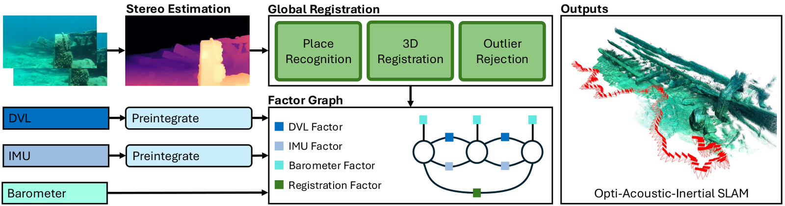
Stereo, trained in simulation and finished on real footage
No large real underwater stereo dataset has ground-truth depth, so the labels come from simulation: eight scenes of wrecks, rocks and vegetation rendered in NVIDIA Isaac Sim in air, with stereo pairs, intrinsics, depth and normals. That is the 105,600-image UWSim set.
Water is added at training time, freshly randomised on every draw. A point light in the camera frame (the ROV's lamps) and caustic textures projected along the normals relight the image; the water-column model above is applied to the relit image, so the added light is attenuated too; sunlight gradients and particles go on last, in image space. The operators need only a stereo pair, depth and calibration, so TartanAir gets the same treatment. FlyingThings3D stays unaugmented, as an in-air reference.
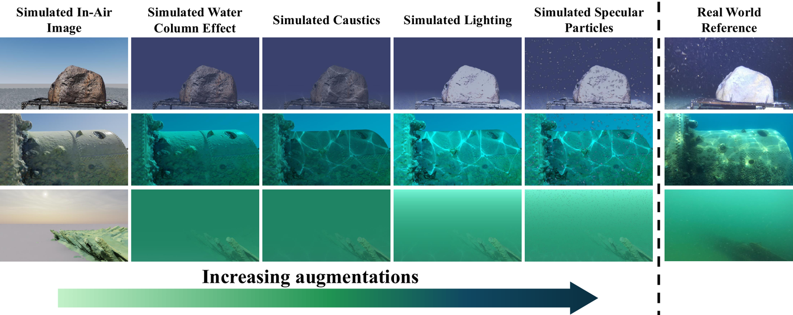
Training has two stages. The first is supervised on simulated data with FoundationStereo's loss, plus one mask: ground truth is dropped wherever , because no network should be asked to recover a surface the water has erased.
The second stage adds real stereo with no labels: 22 sequences from SurfSLAM's own shipwreck surveys (19,950 pairs) plus SVIn2 and Lizard Island footage. The supervision is photometric. Warp the right image into the left camera with the predicted disparity (Kornia does the warp), compare with the real left image under an L1 plus SSIM loss, do the same in the other direction, and average. Where a warped pixel falls outside the other image, only the valid direction counts, at double weight.
Warping cannot fix the water column: when both images are uniform veil, every disparity warps to the same picture. The Occam regularizer is the paper's answer. Compute the photometric loss once more with disparity forced to zero, and penalise a prediction that fails to beat it by a margin (Eqs. 14-15):
The self-supervised loss is ,
the last an edge-aware smoothness term. Table 2 lists , ,
, and a learning rate of
1e-5. The released DEFOM fine-tuning config (config/train/models/defom_stereo/) sets the
margin to 0.1 and the Occam weight to 2.0 instead; the other values match. I did not train
anything, so I cannot say which setting produced the released weights.
The recipe was applied to FoundationStereo and to DEFOM-Stereo at two sizes. DEFOM won, and it
is what SurfSLAM ships: the ViT-L model (382.62 M parameters, 47.30 M of them trainable around a
frozen Depth Anything V2 encoder) for offline accuracy, and the ViT-S model (43.29 M, 18.51 M
trainable) for the SLAM loop, where the released config loads ours_vits_slam.pth.
Stereo is chosen over monocular depth because the baseline makes it metric (the Depth Anything 3 in ROS 2 article shows where a monocular model's metres really come from). Depth is ; with the released calibration's px and m, one pixel of disparity error at 10 m is about 0.62 m of depth (, my arithmetic). Metric, but not precise at range.
Tracking: an acoustic-inertial factor graph
The tracker is TURTLMap (Song et al., IROS 2024), from the same lab, bundled into the SurfSLAM repository. If factor graphs, MAP estimation as nonlinear least squares, or iSAM2 are new to you, the GTSAM 4.3 article builds all of them from scratch; here I only list what goes into the graph.
Each keyframe carries the state (paper, Eq. 17):
orientation and position in a north-east-down frame, body velocity, gyro and accelerometer biases, and a DVL velocity bias, estimated like the IMU's. Keyframes are added at 1 Hz. The sensors arrive at 200 Hz (IMU), 8 Hz (DVL) and 5 Hz (barometer), and between keyframes they are compressed into factors:
- an IMU preintegration factor (GTSAM's
CombinedImuFactor), the same on-manifold integration the FAST-LIO2 article walks through for forward propagation; - a DVL preintegration factor (
VelocityIntegrationFactorinturtlmap/), which rotates each body-frame velocity by the integrated gyro and sums it into a relative translation, keeping Jacobians with respect to the gyro and DVL biases so the optimiser can correct them without re-integrating; - a barometer factor on alone.
The graph is solved incrementally with iSAM2 (Eq. 23). This is smoothing, not filtering: an EKF, as in the Kalman filter article, commits to each estimate and moves on, while iSAM2 keeps the past poses as variables and can move all of them when a late measurement arrives. That property is what makes the next stage worth having.
Stereo as a drift corrector
In the default configuration the camera never enters frame-to-frame tracking
(frame_to_frame: enabled: False). Its output is a registration factor between the
current keyframe and an old one, produced in five steps:
- Place recognition. Equalise the left image with CLAHE, extract SuperPoint features, aggregate them into a VLAD descriptor, and retrieve the three most similar keyframes that are at least 20 seconds old.
- 2D matching. Match with SuperGlue, reject outliers with a RANSAC essential matrix.
- 3D alignment. Lift the surviving matches to 3D with the stereo network's depth, estimate
a rigid transform with RANSAC, and refine it with GICP on the full point clouds
(
small_gicpin the code). - Gate. Compare the transform with the tracker's own belief about the same relative pose, using its marginal covariance, and discard it if the Mahalanobis distance exceeds 2.5. At most one of the three candidates survives.
- Factor. Add the survivor as a between-factor with residual , under a robust kernel so that a bad match that slipped through gets down-weighted rather than trusted.
The whole objective is the acoustic-inertial sum plus the kernel-weighted registration terms (Eqs. 25-26):
Two details of the released code differ from the paper's text. The kernel on stereo factors in
turtlmap/turtlmap/src/Posegraph.cpp is a Cauchy kernel with parameter 2.0, not the Huber
kernel the paper names, and the loop-closure noise is a fixed 0.2 m and 0.1 rad from the config
rather than a covariance from GICP. The default loop-closure gate in cfg/defaults.yaml is 3.5,
compared against the square root of the Mahalanobis form; the paper states 2.5 on the squared
form. None of this changes the idea, but the code the evaluation scripts run is not literally
the equations as printed.
The map
Mapping is deliberately plain. Each keyframe's depth image is back-projected into a point cloud, cleaned on the GPU (edge cleaning, then statistical and radius outlier removal), and placed with the keyframe's optimised pose. There is no fusion volume and no bundle adjustment; the paper names bundle adjustment as future work and notes that large textureless regions make it unstable.
Ground truth in a lake
There is no motion capture around a shipwreck. The reference trajectories and maps come from metric photogrammetry: COLMAP structure-from-motion on the stereo images (5 fps for the SLAM sequences, so it keeps tracking through low texture), then a custom factor-graph optimisation that adds the IMU to recover metric scale and refine the calibration jointly across sequences. For the stereo evaluation sequences the IMU failed in the field, so their scale comes from fixing the stereo baseline at Kalibr's value.
The data were collected at the Thunder Bay National Marine Sanctuary in Alpena, Michigan, by a human-operated BlueROV2 with a forward-facing stereo camera, at depths from 4 to 20 m under natural light, plus an outdoor tank with an artificial rock. The dataset is called SUDS (Stereo Underwater Dataset for Shipwrecks):
| Split | Contents | Ground truth |
|---|---|---|
| Stereo evaluation | 9 sequences, 5 wreck sites, 1,486 pairs | photogrammetry disparity, hand-drawn water masks |
| Stereo training | 22 sequences, 19,950 pairs | none (self-supervision only) |
| SLAM | 3 sequences on one wreck: Boiler 180 s, Engine 284 s, Long 550 s; 29,319 images; 1080p stereo at 30 fps with IMU, DVL and barometer | photogrammetry trajectory and map |
The SLAM configs are named monohansett_boiler.yaml, monohansett_engine.yaml and
monohansett_long.yaml, which points to the wreck. Test data comes from wreck sites not seen in
training. The abstract says "over 24,000 stereo pairs"; I could
not make Table 1's counts sum to that.
The obvious limitation is the one the authors state: the reference is itself built from images, so it only exists where photogrammetry works. Highly turbid water, where the sim-to-real stereo should matter most, cannot be evaluated this way.
The evidence
Stereo: the gain is the water column
Table 3 reports end-point error (EPE, mean disparity error in pixels) and D1 (percentage of pixels off by more than 3 px and 5%), split with the hand-drawn masks into pixels on geometry and pixels in the water column, where the right answer is zero. Lower is better everywhere.
| Model | Combined EPE | Geometry EPE | Water EPE | Water D1 |
|---|---|---|---|---|
| FoundationStereo (ViT-L) | 30.79 | 1.76 | 55.62 | 98.98% |
| DEFOM (ViT-L) | 10.61 | 1.74 | 18.83 | 99.64% |
| SurfSLAM (DEFOM ViT-L) | 1.51 | 1.84 | 1.41 | 5.66% |
| IGEV++ | 23.22 | 1.90 | 43.63 | 99.24% |
| UnderwaterStereo | 25.17 | 7.73 | 41.31 | 98.67% |
| DEFOM (ViT-S) | 4.03 | 2.31 | 6.15 | 91.44% |
| SurfSLAM (DEFOM ViT-S) | 1.68 | 1.79 | 2.05 | 9.58% |
The combined EPE falls from 10.61 to 1.51 px for the large model and from 4.03 to 1.68 px for the small one, and nearly all of it comes from the water column. On geometry the large model is slightly worse than the DEFOM it started from, 1.84 against 1.74 px; the small one improves from 2.31 to 1.79 px, though its BP-1.0 on geometry (pixels more than 1 px off) gets worse, 59.07% against 49.06%. The paper says its models "perform competitively with or better than existing methods" on geometry, which is fair. What the fine-tuning bought is a network that says "nothing here" to open water, which is exactly what a map needs.
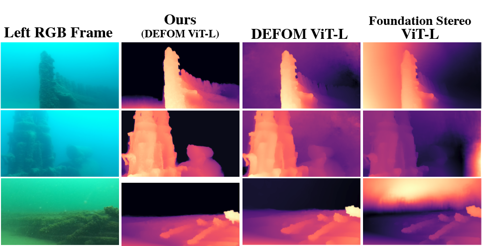
The ablation (Table 4, all DEFOM ViT-L, EPE) says which ingredient does what. Haze-only augmentation leaves the water column at 10.30 px. Adding the full augmentation (light, caustics, particles) takes it to 1.79. The warp loss and in-air data each shave a little more, to 1.41 with everything. On geometry every row sits between 1.84 and 1.91 px.
Trajectories: the DVL carries it
Table 5 gives RMS absolute pose error, the median of five runs. The table prints no unit; the
released evaluation script computes it with evo on the translation part after alignment, so
it is metres.
| Method | Engine (284 s) | Boiler (180 s) | Long (550 s) |
|---|---|---|---|
| DROID-SLAM | 0.164 | 3.121 | 5.794 |
| MASt3R-SLAM (scale-aligned) | 0.395 | 0.462 | 1.963 |
| ORB-SLAM3 | 1.662 | 2.844 | 6.783 |
| SVIn2 | 1.085 | 2.413 | 2.774 |
| TURTLMap (no camera) | 0.399 | 0.528 | 1.312 |
| SurfSLAM | 0.216 | 0.246 | 0.444 |
VGGT-SLAM produced no trajectory on any sequence. DROID-SLAM wins Engine, the most visually rich run, and loses the other two badly. The authors hypothesise that SVIn2 drifts because its IMU initialisation wants the robot at rest; in the field the ROV never was. Versions move: in v2 SurfSLAM's Long number was 0.386, and in v3 it is 0.444.
The sensor ablation (Table 6) is the most informative table in the paper:
| Configuration | Engine | Boiler | Long |
|---|---|---|---|
| everything | 0.216 | 0.246 | 0.444 |
| no barometer | 0.226 | 0.246 | 0.386 |
| no camera (TURTLMap) | 0.399 | 0.528 | 1.312 |
| no DVL | 14.439 | 102.070 | 450.411 |
Without the DVL, the same stereo registrations and IMU produce errors of 14 to 450 m. With the DVL and no camera at all, the error on the 550 s run is 1.312 m. The registrations take that to 0.444 m, about a third. The barometer barely matters, and removing it improves Long; the authors suspect barometer noise or bias fighting constraints that are already sufficient. That is the design argument of the paper in one table: a good acoustic-inertial tracker does the work, and vision is a correction applied when it can be trusted.
Maps: more complete, not more accurate
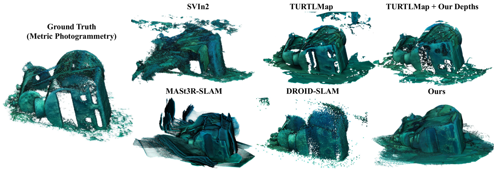
Table 7 scores maps against the photogrammetry at 5 cm resolution: accuracy and completion as mean distances in metres (lower is better), precision and recall as the fraction of points within 0.1 m (higher is better). SurfSLAM wins completion and recall on all three sequences, by a lot: recall 0.96, 0.98 and 0.99 against at best 0.82, 0.79 and 0.62 for the baselines. It does not win accuracy. On Engine DROID-SLAM's accuracy is 0.04 against SurfSLAM's 0.34, and on Long running TURTLMap's trajectory with SurfSLAM's stereo reaches 0.19 against 0.50. The paper reads this as registration trading "a small amount of local accuracy for substantially more complete reconstructions"; on Long, the accuracy cost is not small.
Runtime
"Real-time" here means 1 Hz keyframes, with the acoustic-inertial tracker in between. Table 9 reports stereo inference at 359.3 ± 26.4 ms on the desktop (an RTX A6000 with a Ryzen 5950X) and 786.1 ± 51.2 ms on an NVIDIA Jetson Thor; the graph optimisation takes 6.7 ± 3.4 ms and 9.9 ± 5.1 ms. On the Jetson, 22.8% of input frames are dropped overall, most of them as stale before registration. The Jetson's trajectory error is slightly lower (0.333 m on Long), which the authors attribute to skipping frames that would have produced a bad registration. The Jetson runs replayed sensor data on a bench, not on the vehicle.
What is released
- SLAM code: umfieldrobotics/SurfSLAM, one
commit,
8fc2684, "initial public release" on 18 September 2026, 158 files. Python front end, the TURTLMap C++ backend on GTSAM with pybind11 bindings, Docker setup, the trajectory and map evaluation scripts, and per-scene configs including the sensor ablations. - Stereo code: umfieldrobotics/SurfSLAM_Stereo,
commit
1fa4623of the same day, 127 files: augmentation, training, evaluation and a demo with six bundled stereo pairs. - Data and weights: Deep Blue Data, DOI 10.7302/t2se-wq35,
registered 6 August 2026:
SUDS_STEREO,UWSim,SUDS_SLAM(HDF5 with timestamps, calibration, reference trajectories and maps) andweights/(ours_vitl,ours_vits, the ablation checkpoints and the SLAM checkpoint). The archives are Zstandard with a long window, so they needzstd -d --long=30.
The licensing is less tidy than "public" suggests:
- Neither repository has a licence file at those commits. Code with no licence is visible, not reusable.
- The SLAM repo's submodules are DEFOM-Stereo (MIT) and Magic Leap's SuperGlue, whose licence is headed "ACADEMIC OR NON-PROFIT ORGANIZATION NONCOMMERCIAL RESEARCH USE ONLY". The SuperPoint features and SuperGlue matcher that registration depends on both come from it.
- The ViT-L model is built on a Depth Anything V2 Large encoder, and those weights are CC BY-NC 4.0; the Small encoder is Apache-2.0. The stereo repo also pulls in FoundationStereo, under NVIDIA's own licence.
- The paper itself is CC BY-NC-SA 4.0 on arXiv.
- The Deep Blue record's licence I could not read: the page answered this sandbox with a 403 challenge, and its DataCite metadata carries no rights statement.
For research, everything needed to reproduce the tables appears to be there. For anything commercial, nothing I could verify grants it.
Where it costs
- Evaluation breadth. Three SLAM sequences on one wreck, 550 s at most, and a reference that exists only where photogrammetry succeeds.
- Narrow wins. The stereo gain is the water column; the map gain is completeness, bought with accuracy on Long.
- Hardware. A GPU for stereo at 1 Hz, and a DVL, the one sensor the method cannot do without (Table 6).
- Paper against code. The kernel, the gate and the Occam margin in the release differ from the printed values. Read the configs before quoting the equations.
The one-paragraph summary
SurfSLAM splits underwater SLAM along the line of what each sensor is good at. A DVL, preintegrated with an IMU and a barometer in a GTSAM factor graph, tracks with slow drift. DEFOM-Stereo, fine-tuned on simulated wrecks with water added at train time and then on unlabelled real footage with a warp loss and an Occam penalty, learns to leave open water empty; its depth drives registrations that enter the graph as loop closures, cutting error on a 550 s survey from 1.312 m to 0.444 m, and its keyframe clouds make the map. The stereo gain is almost all water column, the tracking gain is almost all DVL, and the release is complete enough to reproduce and restrictive enough that you should read the licences first.