2026-10-19 · 19 min · 3d · gaussian-splatting · gpu
A 1:50 narrated explainer, drawn in code. Every number and picture in it is this article's own; the sources are below.
› transcript
Hi, I'm Fettle! Today: how a splat renderer that never sorts can still look steady. The new idea is in training. Push every Gaussian on a ray toward one colour, so whichever gets drawn is close to right. The usual renderer sorts by depth and blends a slice of each Gaussian. Sorting costs time, and a flipped order pops. The stochastic renderer skips the sort. Each fragment survives with its alpha, and the depth test keeps one. Right on average, noisy per frame. Here is the formula. P of i is how often Gaussian i wins the pixel, the same weight blending uses. This is how far its colour sits from the pixel's colour. SteadySplats adds this variance to the training loss. Every piece is already computed, so it is cheap. One pixel. Without the term, it blends yellow, dark green and lilac. With it, every band is olive. Both blend to the same colour. Only a stochastic renderer can tell them apart. Each pixel also borrows its neighbours' samples, weighted by how likely each sample is here. Those weights need the occluders in front. A small buffer of recent samples supplies them. Over time, the reuse collapses to a moving average per pixel, the filter temporal anti-aliasing uses. On the paper's camera paths, the variance term alone adds about seven decibels. Reuse does the rest. Sort-free splats do not pop. They boil. Most of the cure is a model whose Gaussians agree. Noise is colour variance along the ray. A loss term shrinks it, and reuse cleans up the rest. Every source is in the full article. I'm Fettle. Bye!
Why read this
Notabletop 60%Measures the variance term on the released bonsai model vs original 3DGS with a from-scratch compositor; corrects the popping framing.
- Original analysis
- A lasting reference
- A new technique
3D & spatialRuns on a consumer GPUResearch paper
How this was scored
- Is it new?
- 2 of 3: A real new idea, method or capability
- Can I trust it?
- 2 of 3: Measures key facts from files, code or configs
- Can I run it?
- 1 of 3: API-only, gated or restrictive licence
- Will I understand it?
- 2 of 3: Mechanism from first principles with figures
- Can I act on it?
- 2 of 3: A concrete recipe, numbers or comparison
- Will it last?
- 2 of 3: A reference for a year or more
- Does it affect many?
- 1 of 3: A specialist community
- Only here?
- 2 of 3: A teardown or measurement few others did
Score 63 of 100, ranked 241 of 577 rated articles. Each question is answered 0–3 by hand, and a 3 is rare. How articles are scored
The post that sent me here is Sameh Khamis's: "I have SteadySplats implemented in the browser! Saw this tweet yesterday - had it working today, couldn't wait for the code release! Training is unaffected - new variance term is practically free. Rendering is at a solid 240 fps throughout, bigger difference with denser views." The tweet he saw is Radiance Fields', whose reply links the paper, arXiv 2610.05576, and the project page.
It is easy to read "steady" and "variance term" as a cure for popping, the flash you see when a sorted splat renderer reorders two overlapping Gaussians as the camera moves. That is not what this paper fixes. SteadySplats renders without sorting at all, so there is no order to flip. What it fixes is the price you pay for not sorting: noise. This piece is about where that noise comes from, the one-line training term that removes most of it, and the resampling filter that cleans up the rest. I checked the variance term on the authors' own released model.
Numbers are labelled measured (I computed them from a file or a run of my own code), reported (the paper's or a poster's figure, not re-run) or reasoned (my arithmetic on the other two).
Sorted, popping, or noisy
A 3DGS renderer colours a pixel by walking the Gaussians that cover it front to back. Gaussian has colour and, at this pixel, an alpha . Its weight is its alpha times the light that got past everything in front of it:
That needs an order. The original renderer sorts Gaussians once per tile by the depth of their centres, which is cheap but wrong whenever two Gaussians overlap in depth: nudge the camera, the centre order flips, and a pixel's colour jumps. That jump is popping. StopThePop removes it by sorting per pixel by the depth of each Gaussian's peak response, at a cost in speed. The sort itself is the other cost: millions of keys, every frame, which is the frame-time dial on phones.
Stochastic transparency throws the sort away. Draw every fragment opaque with depth testing on, but keep fragment only if a random number falls below . Fragment is the one you see when it survives and everything in front of it does not, which happens with probability , exactly its blending weight. The z-buffer does the ordering for free. This is the StochasticSplats estimator the paper builds on; Blender 5.3 does the same thing with rays in Cycles, and PlayCanvas ships it as a WebGPU flag.
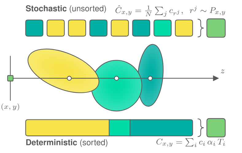
One sample is one Gaussian's colour, not the blend. The expected value is right; any single frame is wrong by however far that Gaussian's colour sits from the blend. The paper writes the root-mean-square error of an -sample estimate as
At one sample per pixel and uncorrelated noise between frames, this is not popping; it is a boiling, sparkling image. The usual answer is to raise by accumulating frames, which ghosts when the camera moves and undoes the speed you bought by not sorting. The paper's insight is to go after the other factor.
The variance term
Nothing in standard 3DGS training cares about . The photometric loss only sees . So the optimiser is free to hit a pixel's olive green by stacking a pale yellow Gaussian, a near-black one and a pinkish one at half opacity, and it often does: semi-transparent "fuzz" layered over a surface is how 3DGS buys fine detail and view-dependent effects. A sorted renderer cannot tell that pixel from one made of four olive Gaussians. A stochastic renderer can, because every sample is one of those colours.
SteadySplats adds the variance to the loss (Eq. 7), averaged over the pixels of the training view:
is the blending weight the rasteriser already computes. The paper swaps the rendered colour for the ground-truth pixel , which is cheaper and, for a converged model, the same thing. The effect is that every Gaussian covering a pixel is pulled towards that pixel's colour.
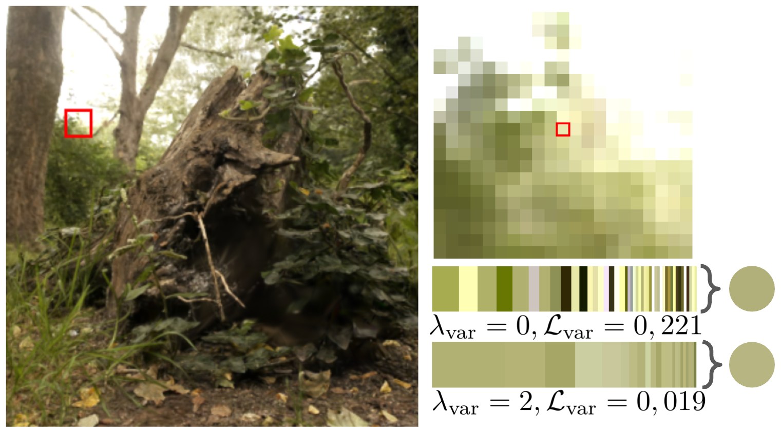
Here is that pixel as a toy. The slider walks between two fits I made up that blend to the same colour; the strip shows what a one-sample renderer would put on screen in successive frames.
The plain fit has a variance of 0.2885, which at one sample per pixel is a PSNR of about 10.2 dB against the sorted colour; the regularised fit has 0.0041, about 28.6 dB (reasoned, from the toy's own numbers, which are illustrative). Going from 1 to 64 samples buys dB (reasoned). The variance term buys more than that here without drawing a single extra sample, which is the whole pitch.
Why it is cheap to train
Sameh says the term is "practically free", and the structure says why (reasoned). The forward pass already walks each pixel's Gaussians and has and in registers; adds one more running sum. The paper's gradients (its Section 13) are , and for a term in minus a suffix sum over the Gaussians behind . The 3DGS backward pass already walks back to front carrying exactly such a suffix sum for the colour gradient, so this is one more accumulator per pixel, not a new pass. I could not measure the overhead: the released training logs cover only the regularised second half of training, with no baseline run on the same machine to compare against.
What it does to the model, measured
The authors publish their models for seven Mip-NeRF 360 scenes, with the training config and TensorBoard logs. The original 3DGS bonsai model by Kerbl is in the dylanebert/3dgs dataset (revision 703d19c, the same file the Blender article sampled). Both use the same COLMAP frame: camera 0 in each cameras.json sits at the same position to 15 digits. I parsed both PLYs in full (measured):
| bonsai, iteration 30,000 | original 3DGS | SteadySplats, |
|---|---|---|
| Gaussians | 1,244,819 | 1,107,934 |
| median opacity | 0.197 | 0.894 |
| opacity above 0.99 | 14.52% | 42.02% |
| opacity below 0.01 | 16.47% | 11.36% |
| median largest-axis scale | 0.0306 | 0.0353 |
The paper reports that the term "naturally acts as a binarization penalty on opacity" (Figure 11). On bonsai that is not subtle: the typical Gaussian goes from mostly transparent to nearly opaque.
To measure the variance itself I wrote a small CPU reference of 3DGS compositing in NumPy: project each Gaussian with the EWA Jacobian and the 0.3-pixel dilation, evaluate degree-3 spherical harmonics, sort each pixel's fragments by depth, composite front to back with the 3DGS early exit at transmittance , and accumulate per pixel, counting the black background as a sample with whatever mass is left. It also draws one stochastic sample per pixel from . I rendered test camera 0 (DSCF5565) at the training resolution, 1559 x 1039 pixels, on a shared 4-core VM, CPU only (measured):
| test view 0, full frame | original 3DGS | SteadySplats |
|---|---|---|
| mean per-pixel | 0.0693 | 0.0065 |
| median per-pixel | 0.0492 | 0.0029 |
| predicted 1-sample PSNR vs sorted | 16.4 dB | 26.7 dB |
| simulated 1-sample PSNR vs sorted | 16.7 dB | 26.7 dB |
| expected occluders in front of the sampled Gaussian | 14.7 | 10.2 |
| fragments blended before early exit | 48.6 | 41.8 |
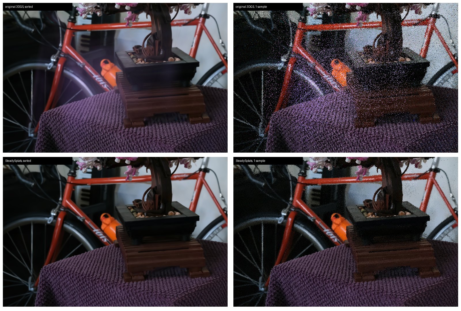
Variance down by a factor of 10.7 is 10.3 dB at one sample per pixel (reasoned). The predicted and simulated PSNRs agree, which is the check that the variance formula and the sampler are the same thing. The occluder count matters for the next section: SteadySplats' resampling weights need the Gaussians in front of a sample, and they only stay cheap when there are few. The term cut the expected occluders from 14.7 to 10.2, the direction the paper's Figure 16 shows. It also cut the number of fragments blended before early exit, from 48.6 to 41.8, where the paper's Figure 16 has that number going up with ; my baseline is Kerbl's original model rather than the authors' own run, and this is one view of one scene, so I would not read much into it. Also not comparable: the paper's variance axis uses the ground-truth colour, which adds the model's own error, while mine uses the rendered colour, so mine is smaller by construction.
A caution on the bright specks in the original model's one-sample image. Many are Gaussians whose colours are far outside the blend: bright, mostly hidden layers that a sorted renderer attenuates to nothing and a stochastic one occasionally shows in full. The paper notes the term "reduces the number of bright primitives, which are often floater artifacts" (its Figure 15).
The rest of the pipeline
The variance term changes the model. Two more pieces change the renderer.
History-based spatial resampling. Neighbouring pixels see nearly the same Gaussians with nearly the same weights. So pixel also uses the sample its four neighbours drew, weighted by how likely that sample is at compared with where it was drawn: , then normalised (self-normalised importance sampling). A sample from across an edge gets a small weight and does not blur it; a plain 3x3 blur would. The ratio splits into the Gaussian's own alpha at the two pixels, which is easy, and the change in what occludes it, which needs to know what is in front, which is exactly what a sort-free renderer does not have. The trick: keep a small per-pixel buffer of the distinct Gaussians sampled there recently, with their depths, and take the occlusion product over only those. With the variance term on, the few dominant occluders are the ones most likely to have been sampled, so a small buffer catches them.
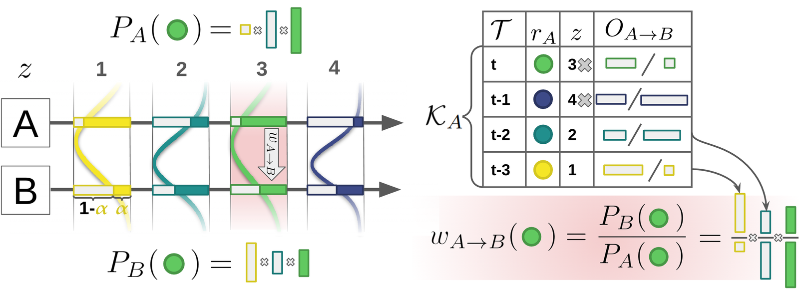
Temporal reuse as an EMA. The same weighting extended over past frames would need every old sample. The paper proves (Theorem 1) that if every history sample decays by a shared factor per frame, the full spatio-temporal estimator collapses to a two-number recursion per pixel; at steady state it is the familiar exponential moving average of temporal anti-aliasing, , with in the evaluation (reported). StochasticSplats' cumulative average and Gaussian Point Splatting's fixed EMA fall out as special cases. Instead of clamping the history colour as TAA does, which clips legitimate Monte Carlo tails, SteadySplats lowers smoothly when the reprojected history is far from the current neighbourhood. Samples are drawn from spatio-temporal blue noise, offset per primitive, rather than white noise.
Results, against what
The comparison is to the other sort-free renderers, StochasticSplats and Gaussian Point Splatting, with sorted 3DGS as ground truth. StopThePop is in the related work, not in the tables: it is a sorted renderer and does not have this noise. All of the following is reported.
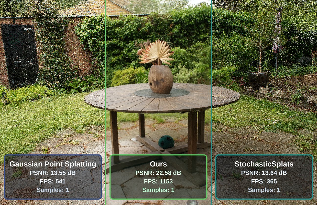
On a camera-path benchmark of 21 trajectories and 3,152 frames over 7 Mip-NeRF 360 scenes, rendered at 1 sample per pixel and scored against sorted rendering of the same path (Table 1):
| method | avg PSNR | SSIM | LPIPS | tPSNR |
|---|---|---|---|---|
| StochasticSplats | 18.336 | 0.293 | 0.667 | 15.235 |
| StochasticSplats + temporal | 21.954 | 0.552 | 0.524 | 19.450 |
| SteadySplats, no temporal | 31.437 | 0.845 | 0.345 | 28.410 |
| SteadySplats + temporal | 35.085 | 0.937 | 0.209 | 32.449 |
tPSNR is PSNR on frame-to-frame differences, the flicker metric. 31.437 minus 18.336 is 13.1 dB, which is the abstract's "13 dB" (reasoned). The ablation (Table 2) isolates the training term: alone takes average PSNR from 18.336 to 25.561, a 7.2 dB gain (reasoned), and tPSNR from 15.235 to 22.423, more than spatial reuse alone (24.774) or temporal reuse alone (25.227). All three together are best. My bonsai frame, with the variance term and no reuse at all, sits at 26.7 dB, the same regime as that 25.561 (reasoned; one view of one scene, not their benchmark).
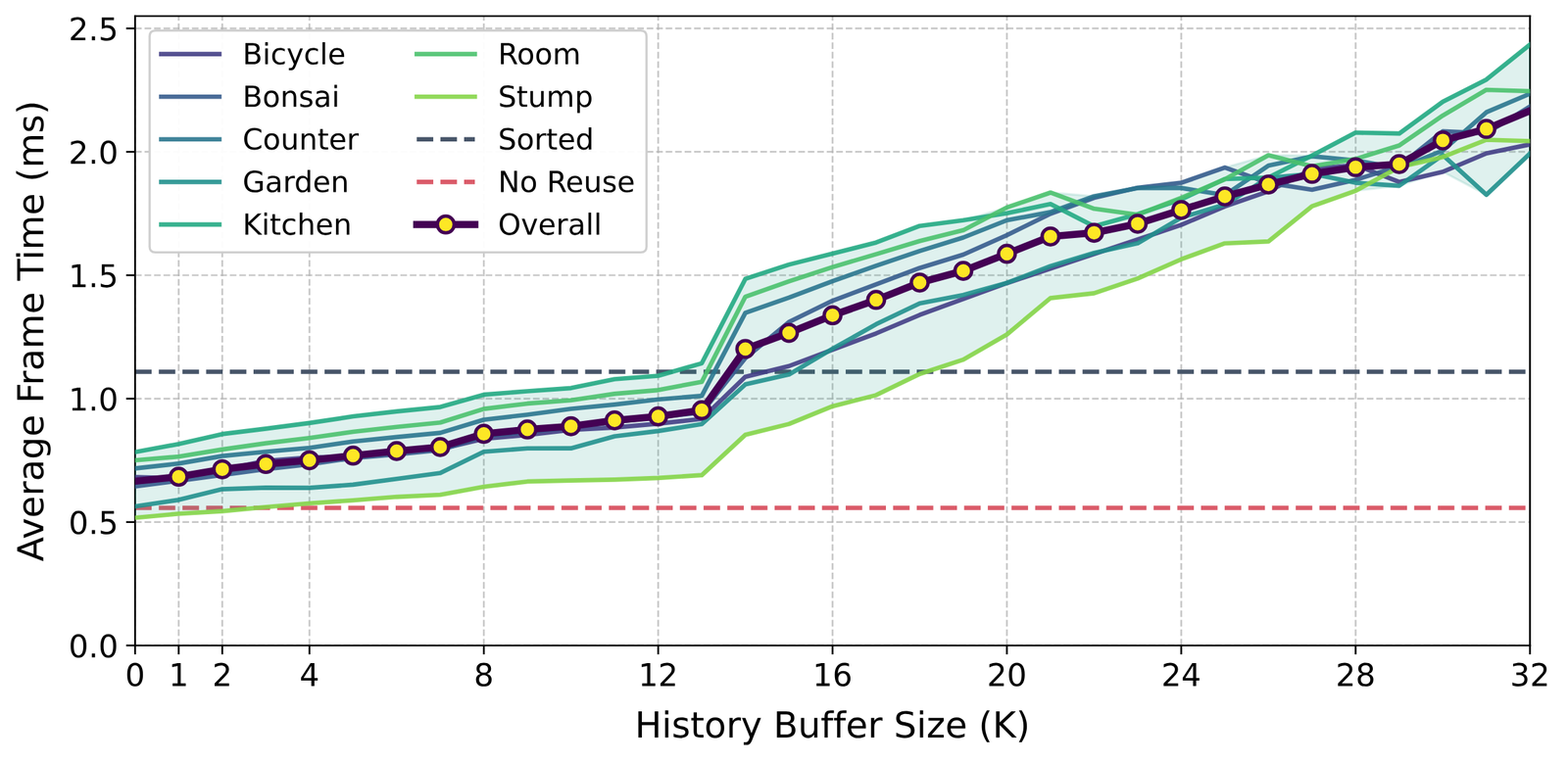
Speed is on an RTX 5090 in the authors' Vulkan renderer. Their Figure 7 puts plain stochastic rendering near 0.56 ms a frame and sorted blending near 1.11 ms, with spatial reuse rising slowly from about 0.7 ms and staying under the sorted line until the buffer size reaches 14, where shared memory fills and the cost jumps (reported, read off the plot). They use . Their "excess quality factor", the multiple of samples resampling is worth at equal time, peaks at 3.5 at low sample counts. And on convergence: with , matching the PSNR of 31 samples at takes 256 samples at .
What it costs
Peak quality. The paper says so in its limitations: "dilutes the training signal", giving "a slight decrease in peak quality metrics", and there is a floor near below which quality collapses. Its Figure 5(a) plots deterministic PSNR against variance for each scene; the bonsai curve starts near 31.9 dB at (reported, read off the plot). The released bonsai model's own log records a test PSNR of 30.68 dB at iteration 30,000 (measured, from the published TensorBoard file). That is about 1.2 dB below the plot's unregularised point (reasoned), more than "slight", although the plot labels only its first and last points, so I cannot tell which of its points the released model corresponds to. The other released logs (measured):
| scene | test PSNR, | Gaussians | median ms per iteration, 15k to 30k |
|---|---|---|---|
| bicycle | 24.63 | 4,356,410 | 31.0 |
| bonsai | 30.68 | 1,107,934 | 22.5 |
| counter | 28.38 | 1,031,498 | 23.9 |
| garden | 26.45 | 3,337,046 | 25.2 |
| kitchen | 30.43 | 1,429,953 | 25.5 |
| room | 31.38 | 1,290,097 | 29.0 |
| stump | 25.34 | 3,714,063 | 23.2 |
Every config trains at the Mip-NeRF 360 convention, indoor scenes at half resolution and outdoor at quarter. The iteration times are the authors' GPU, not mine, and with no baseline log they say nothing about the term's overhead.
Bias. Plain stochastic transparency is unbiased. Resampling is not: the self-normalised estimator has bias, the occlusion product misses occluders that were never sampled into the buffer (worst at silhouettes and thin structures), and a neighbour across a 16x16 tile border can borrow a Gaussian the tile never rasterised, which the paper bounds at alpha below 1/256. The paper still reports convergence to sorted 3DGS at an average L1 error under .
A changed model. The variance term is a training-time change, so you cannot apply it to a splat you already have. The renderer side (resampling, EMA, blue noise) works on any model, but its occlusion approximation leans on the model having few occluders, which is what the training term provides.
Sameh's browser version
There is no code from the authors yet; the project page says "Code coming soon". Sameh Khamis had not published his implementation either when I checked, so everything here is reported, read from his post and its 106-second video.
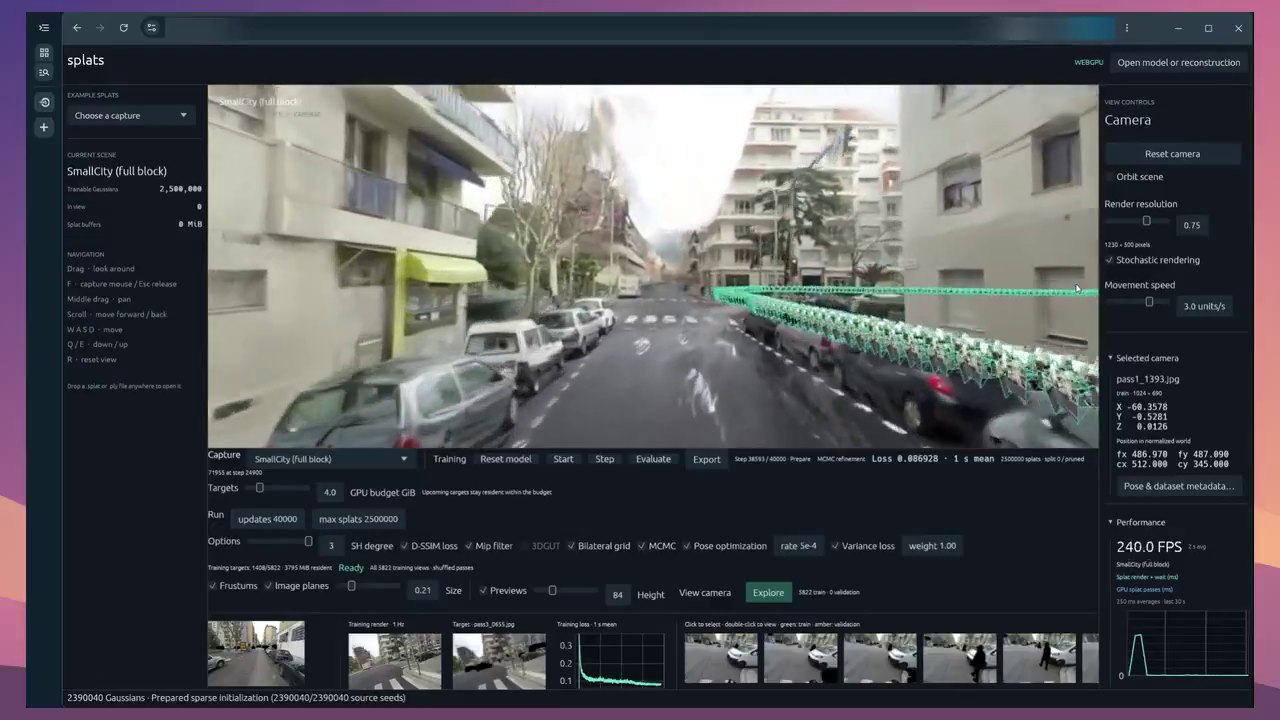
The video shows a WebGPU app called splats that trains as well as renders. The capture is "SmallCity (full block)" with 2,500,000 trainable Gaussians, 40,000 updates and MCMC densification, plus a bilateral grid and pose optimisation. "Variance loss" is a checkbox with weight 1.00, the paper's ; "Stochastic rendering" is a separate toggle in the viewer, at 0.75 render scale, 1230 x 500 pixels. So his "training is unaffected" is about cost; the model is trained with the term, as the paper requires.
On the 240 fps: the readout sits at exactly 240.0 FPS whenever training is not running and drops to the 20s to 40s while it is (37.7 FPS at step 11,700). A frame rate that flat and that round is most likely a 240 Hz display's vsync cap, not the renderer's throughput (reasoned). A reply asked exactly this and was not answered; he did say the GPU is a 3090 Ti. "Bigger difference with denser views" is not explained in the thread, so I will not guess.
Takeaways
- SteadySplats is about noise, not popping. The renderer it improves never sorts, so it never pops; it boils. If popping is your problem, the answer is still a per-pixel sort like StopThePop, or going sort-free and paying in noise.
- Most of the win is in the model, not the renderer. One loss term, already computable from the forward pass, pushes every Gaussian on a ray towards the pixel's colour. On bonsai it cut the measured per-pixel variance by a factor of 10.7 and turned the median Gaussian nearly opaque.
- It is not free in quality. The released bonsai logs 30.68 dB, and the paper itself names a variance floor and a peak-quality trade.
- Resampling is ReSTIR's idea in splat clothing, made cheap because the trained model has few occluders, and its temporal half is an EMA you already have.
What I could not check: I did not run the authors' renderer (unreleased) or reproduce any table; my compositor is an independent reference with no reuse, so it measures the training term only. Figure 7 and Figure 5(a) values are read off plots. Sameh's implementation is known only from his video.
Related: the sort-free trick and its noise on phones are in Gaussian-splat capture in practice; the ray-traced version is in Blender 5.3's Gaussian splats; what the opacity of a splat does for cleaning a feed-forward scene is in InfiniSplat v2; how splats are shipped to browsers at all is in the SOG format; and a lidar-fused capture you might render this way is in Hesai Kosmo.