2026-10-13 · 24 min · world-models · video-generation · diffusion · distillation · kv-cache · realtime · lora
Why read this
Notabletop 60%Reads the streaming CWM code end to end: the causal mask, the RoPE-moved cache, a history kept at noise 0.625, and why 5.1 s per 0.71 s chunk is not live.
- Interactive explanations
- Original analysis
- Concrete numbers to act on
Image & video generationNeeds datacenter GPUsNo licenceResearch model
How this was scored
- Is it new?
- 1 of 3: An incremental tweak
- Can I trust it?
- 2 of 3: Measures key facts from files, code or configs
- Can I run it?
- 1 of 3: API-only, gated or restrictive licence
- Will I understand it?
- 3 of 3: Mechanism carried by interactives built from real code or data
- Can I act on it?
- 2 of 3: A concrete recipe, numbers or comparison
- Will it last?
- 1 of 3: Relevant for months
- Does it affect many?
- 1 of 3: A specialist community
- Only here?
- 2 of 3: A teardown or measurement few others did
Score 59 of 100, ranked 292 of 513 rated articles. Each question is answered 0–3 by hand, and a 3 is rare. How articles are scored
Yesterday I took apart StreamRender-H3, NVIDIA's racing game in which code runs the world and a 33B video model paints it. A day later Tingting Liao posted the research-lab version of the same bet: "We made Code World Model causal: video is generated chunk by chunk from a live proxy. A 4-step distilled model renders each chunk in ~5 s on one H200." Code and two checkpoints are open.
Two words in that post made me want to read the code. "Live" and "~5 s" do not obviously belong in the same sentence. A chunk here is 17 frames, which plays for 0.708 seconds at 24 fps, so five seconds to render one is about seven times slower than the video it produces. I wanted to know what "live" means in that case, and what it took to make a model that was trained on whole five-second windows work one chunk at a time.
The short answer is that "live" describes the model's information flow, not its speed. Every chunk is generated from the proxy up to that chunk and nothing after it, and that property is built with real care. The README is honest that the speed is not there yet: its highlights say "5.1 s per chunk on one H200 (not yet real time)". What the README doesn't spell out is what that gap does to a live loop, or what a few of the cleverer choices in the sampler cost, and most of this piece is about those two things.
- branch
- main
- tests
- 10 files
- source
- 244.5 kB
- commit date
- 2026-10-12
by size of tracked source at this commit, file counts in brackets; docs, data and vendored trees excluded
local clone, 2026-10-13 at 64c489a — branch, commit, commitDate, fileCount, hasTests, languages, shallow, testFileCount
shallow clone: counts describe the pinned tree, not the history
What Code World Model was
The base is Code World Model (CWM), from Yiwen Chen, Guosheng Lin and Chi Zhang at Westlake and NTU, posted in August with code and a LoRA. Not to be confused with Meta's CWM, a 32B code-generation language model with the same name and nothing else in common.
The paper's argument is that video world models learn the wrong thing from pixels. They see outcomes, not the rules that produce them, so a door opened in one clip is shut again thirty seconds later. CWM splits the job. A coding agent is the "world brain": it reasons about what should happen and writes code that keeps the world state (positions, health, inventories, timers) in ordinary data structures, where a door stays open because a boolean says so. A small compiler turns that state into a proxy video, and a video model renders the proxy into photoreal frames.
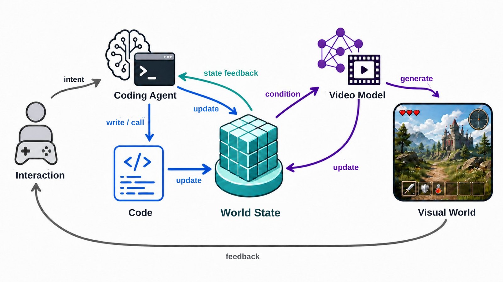
The video model is MiniMax H3, the 33B omni-modal generator, in its Ref2VA mode: a reference picture, a reference video and a caption go in, a 124-frame clip at 1344x768 comes out. CWM fine-tunes it with a rank-128 LoRA on all 50 blocks, about 596M trainable parameters by the paper's count, on 5.6 hours of GTA V gameplay paired with proxies extracted from the game's own runtime.
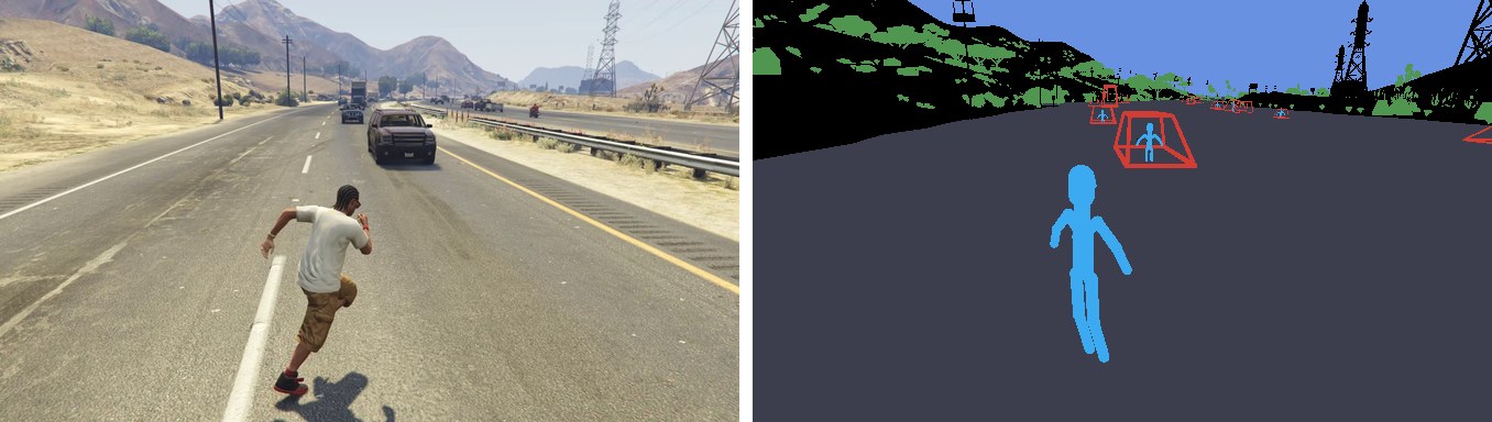
The proxy is the interface that everything in the streaming work is built around, so it is worth knowing exactly what it is. In the released inference code (src/cwm_h3_inference/duv.py) every proxy frame is two files at 336x192: a float32 depth map in metres and an 8-bit semantic-ID map with 12 classes (void, sky, water, terrain, paved road, vegetation, building, infrastructure, human, animal, vehicle, prop). The loader packs them into a three-channel image it calls DUV. Depth is clipped to 0.3 to 256 m and log-encoded into 16 bits. The class ID is split across the other two channels: class % 4 picks one of four U values and class // 4 one of three V values. The result looks enough like an image that H3's own video VAE can encode it, and it does, into a 12x21 latent grid per latent frame (padded to 22), a sixteenth of the 48x84 grid of the target video.

The paper's conclusion has the sentence this whole repository answers: "We also do not implement autoregressive real-time generation." The released sampler couldn't, for three reasons I found in its INFERENCE.md and constants. It denoises a 124-frame window all at once, bidirectionally, so frame 0 of a window attends to proxy frame 123, about 5.1 seconds in the future. Long videos are windows overlapping by 34 frames, each advancing by 90. And each window's caption carries an "action timeline", a text description of what the protagonist is about to do. A game can't hand over five seconds of proxy it hasn't computed yet, let alone a script of the player's next moves.
A chunk is one VAE clip, and that choice does a lot of work
The first design decision is the size of a chunk, and it is the right one. H3's video VAE encodes independent 17-frame clips into 5 latents each. So rtcwm/model/layout.py:17 makes a chunk exactly one such clip: 5 latents, 17 frames, 0.708 seconds. Because the VAE never mixes clips, encoding chunk k's proxy or decoding chunk k's video never needs a frame from chunk k+1. Any other chunk size would have needed a causal VAE, or a lookahead, or a hack at every boundary.
Each chunk is generated inside an attention span of itself and the five chunks before it (SPAN_CHUNKS = 6, line 19), 30 latents or 4.25 seconds. The span is packed as a standalone H3 sequence, in the same layout the released Ref2VA model was trained on: caption tokens, the start image, the six proxy chunks, an audio track (silent, but H3 insists on one), then the video chunks.
Positions are where a naive streaming port goes wrong. H3 uses rotary embeddings on a time axis, and the released model has only ever seen positions inside one 124-frame window. If chunk 80 sat at time position 80 chunks, it would be far outside anything the model knows. So positions are counted from the span's first chunk. Chunk 80 is generated at position 5, like chunk 5 was.
That creates a cache problem. The keys of chunk 79 were computed when it sat at position 5; now it needs to sit at position 4. The sampler doesn't recompute them. It rotates them. _shift_time in rtcwm/model/sampler.py:209 has a one-line docstring that carries the idea: "RoPE rotations compose, so rotating the keys of position p by delta gives exactly the keys of position p + delta (values carry no position)." When the span slides by one chunk, the oldest chunk is dropped and every surviving chunk's keys get rotated back one chunk's worth of time. By default the rotation is not even stored: ROTATE_IN_ATTENTION = True keeps one copy of each cached key and applies the pending shift inside the attention call.
Then the mask. This is the whole of the causality, and it is short enough to quote (rtcwm/model/masks.py:35-39):
if qr == STATIC:
    return kr == STATIC or (static_sees_first and kc == 0 and kr in (DUV, VIDEO))
if qr == DUV:
    return kr == STATIC or (kr == DUV and kc <= qc)
return kr == STATIC or (kr == DUV and kc <= qc) or (kr == VIDEO and 0 <= qc - kc < SPAN_CHUNKS)
Read it as three rules. The static rows (caption, start image, audio) see each other. A proxy chunk sees the static rows and proxy chunks up to itself. A video chunk sees the static rows, proxy chunks up to its own index, and the video chunks of its span. The widget below draws that rule for whichever chunk you pick, next to the released model's dense window.
There is one exception in the mask that I would have missed without the docstring. In the first span of a stream, the static rows also see chunk 0 of the proxy and the video, because that is how the released model's conditions behave: with no history, chunk 0 needs condition rows that look at it. Once there is a history, the conditions see only themselves. The comment says that does better, and I have no reason to doubt it, though there is no ablation to check.
The text side was made causal too, which is easy to forget. In CWM, the Qwen3-VL encoder that turns the caption into conditioning also looks at proxy frames, every 12th frame of the window. In the streaming version (rtcwm/train/preencode.py:251) Qwen sees the start image and the start frame's proxy repeated, "nothing of later frames", and the caption is cut to its "Appearance and scene" section, without the timeline. So the text describes who is in the scene and what it looks like. Everything that moves comes from the proxy.
A consequence of the 6-chunk span is that the model's visual memory is short. A chunk sees 3.54 seconds of earlier video. Anything that left the frame before that is gone from its view, and only the start image, the caption and the proxy know about it. I don't think that's a flaw in this design. It is CWM's thesis showing up in the architecture: persistence lives in the code's world state, and the renderer only has to be consistent for a few seconds at a time. Whether that holds up when a character walks back to a building it saw a minute ago is exactly what I'd want to see tested, and the repo doesn't test it.
The data: CARLA, made deliberately worse
To fine-tune for streaming you need long videos with proxies, and GTA V clips are not something you can regenerate at will. The repo renders its own in CARLA: a pedestrian walking a route through a town, followed by a third-person camera, 934 frames per render. After quality control, data_lists/clips.json keeps 342 clips and drops 1, which at 934 frames and 24 fps is 3.7 hours. Another 201 caption windows across 90 clips are flagged as bad and excluded from training spans.
The interesting decision is the proxy. CARLA can give you perfect depth and segmentation of the real meshes, and the repo throws that away. rtcwm/data/proxy.py rebuilds a coarse proxy from the scene's description using the primitives and ray tracer of open-code-world-model, a separate proxy compiler by Guangyi Liu: buildings become their level bounding boxes trimmed clear of the walking path, poles become capsules, vegetation becomes lobed clumps, roads become flat strips from lane waypoints, and the protagonist is a generic human rig with "position, heading and a procedural gait only -- no body shape or clothing". Its docstring gives the reason in one line: "At test time a coding agent only has coarse geometry, which is what CWM's proxy is."
I like this a lot. Training on the exact segmentation would have produced a model that looks great on CARLA and falls apart when an agent's boxy, approximate world shows up. Training on the proxy you will actually get at inference is the unglamorous choice that makes the open-world results in the video above possible at all.
Teaching it not to trust its own past
A causal video model trained on clean history learns to copy that history faithfully. At inference the history is its own output, slightly wrong, and copying it faithfully means compounding the error. Exposure bias, in other words, and the repo attacks it twice.
The first pass is diffusion forcing. During training every chunk of a span gets its own independent noise level, so the model routinely predicts chunk 4 from a chunk 3 that is half noise. The noise levels come from df_levels (rtcwm/model/objectives.py:66), drawn uniformly and flow-shifted with shift 3, and its docstring records a failed experiment: "History chunks are never the clean ground truth: a clean ground-truth history teaches the model to trust its history completely, which it must not do with its own (imperfect) history at inference (v3 drew one with probability 0.5 and drifted more)." A useful negative result, written down where the next person will find it.
The diffusion-forcing run starts from the released CWM LoRA and trains for 5 epochs; the README budgets 8 nodes for about 7 hours. The released streaming_df.safetensors carries step: 1118 in its metadata. Sampled with 35 Euler steps, it is the slow model in the results table.
Four steps, and a history that stays noisy
The second pass is distillation, and it follows CausVid and Self Forcing closely. rtcwm/train/distill.py stacks three LoRAs on one frozen H3: a student (initialised from the diffusion-forcing model), a frozen teacher, and a critic. Each iteration the student streams 8 to 14 chunks on its own output, the way it will at inference, with each chunk stopping at a randomly chosen one of its four steps. The last four chunks of the teacher's window keep their gradient graph. The teacher scores where that rollout should go, the critic learns where the student actually goes, and the student is pushed along the difference, which is the DMD gradient (distill.py:175-178):
p = x.detach() - x0_real
grad = (x0_fake - x0_real) / p.abs().mean().clamp_min(1e-6)
stack.use("student")
return 0.5 * torch.nn.functional.mse_loss(x.float(), (x.detach() - grad).float()), ...
The critic gets 7 updates for every student update, all on windows cut from the same detached rollout, because the rollout is the expensive part. There are two choices of teacher. With --teacher-kind released it is the original CWM, run bidirectionally on a 37-latent window, exactly as released. With --teacher-kind causal it is the streaming diffusion-forcing model itself, on the student's own six-chunk span. The README's training command uses the causal teacher, initialises the student from step 800 and the teacher and critic from step 1118, and runs --iters 100. The released streaming_dmd_4step.safetensors says iter: 100 and objective: dmd-4step in its header. A hundred iterations is a short distillation; it is also enough to beat the 35-step model on the metric they report, which tells you how far the 35-step model had drifted.
The student samples with the "x0" rule: each step predicts the clean chunk, then re-noises it to the next level with fresh noise. At shift 5, four steps visit noise levels 1, 0.9375, 0.833 and 0.625 before the final clean prediction, and distill.py:64 has the same schedule in a comment. The widget lets you move the shift and the step count.
The detail I didn't expect is what goes into the cache. A finished chunk has to enter the KV cache so later chunks can attend to it. The obvious way is one more forward pass over the clean chunk. The sampler's default, HISTORY_FROM_LAST_STEP = True (sampler.py:166), skips that pass and caches the keys and values the chunk's rows already had in its last denoising step. That step's input was at noise level 0.625. So every chunk a later chunk looks back at is, in effect, a fairly noisy version of itself.
That saves one of five transformer passes per chunk, and the comment claims a second benefit: "the noisy history damps the drift of a long rollout". It fits the diffusion-forcing story, where the model was trained to read noisy history with suspicion. The distillation rollout is set up to match (--rollout-history last-step noises the history to the same level), so the student is trained on the history it will actually see. I'd still like the comparison. --no-history-from-last-step exists for exactly that, and the README doesn't report it.
The other speed trick, --kv-reuse, is also on in the README's 4-step command. Without it, the sampler re-runs the whole history of the span every chunk, which is exact. With it, history keys and values are kept from when they were first computed and only rotated. The module docstring is upfront that this is "an approximation of the exact default": those keys were computed in an earlier span, against a different window of history and conditions. tests/test_kv_reuse.py checks that rotating in attention matches rotating a copy, to within 0.02; there is no test of reuse against the exact re-run. The headline 4-step numbers are all with reuse on.
What 5.1 seconds buys
The README's results are four held-out CARLA clips, 24 chunks each (17 seconds), one seed, scored by pixel MSE against the ground-truth render:
| model | steps | mean MSE | 0-4 s | 13-17 s | s / chunk |
|---|---|---|---|---|---|
| streaming diffusion forcing | 35 | 2231 | 1335 | 3332 | 47.9 |
| + DMD, released CWM as teacher | 4 | 1741 | 1049 | 2501 | 5.2 |
| + DMD, streaming model as teacher | 4 | 1660 | 1070 | 2555 | 5.1 |
The 4-step student is 9.4 times faster than the 35-step model (47.9 / 5.1), which the README rounds to "9×", and its mean MSE is about 26% lower. Distillation improving quality is the usual Self Forcing result: the student was trained on its own rollouts, the teacher never was.
Look at the drift, though. From the first four seconds to the last four, the 35-step model's error grows 2.5 times (1335 to 3332). The best 4-step model's grows 2.39 times (1070 to 2555). Distillation lowered the whole curve without flattening it much. And between the two teachers the order flips by time: the released-CWM teacher is better in both the first and last windows, the streaming teacher wins on the mean. With one seed and four clips, I wouldn't read anything into an 81-point gap.
I'd also be careful with pixel MSE itself. A mean of 1660 on 0-255 pixels is an RMS error of about 41 levels per channel. Against a CARLA render, a model that blurs every texture scores better than one that invents a sharp, plausible, different texture, so MSE rewards a smoother sampler. It does catch the failure that matters most here, drift away from the scene, and nothing else in the repo measures quality.
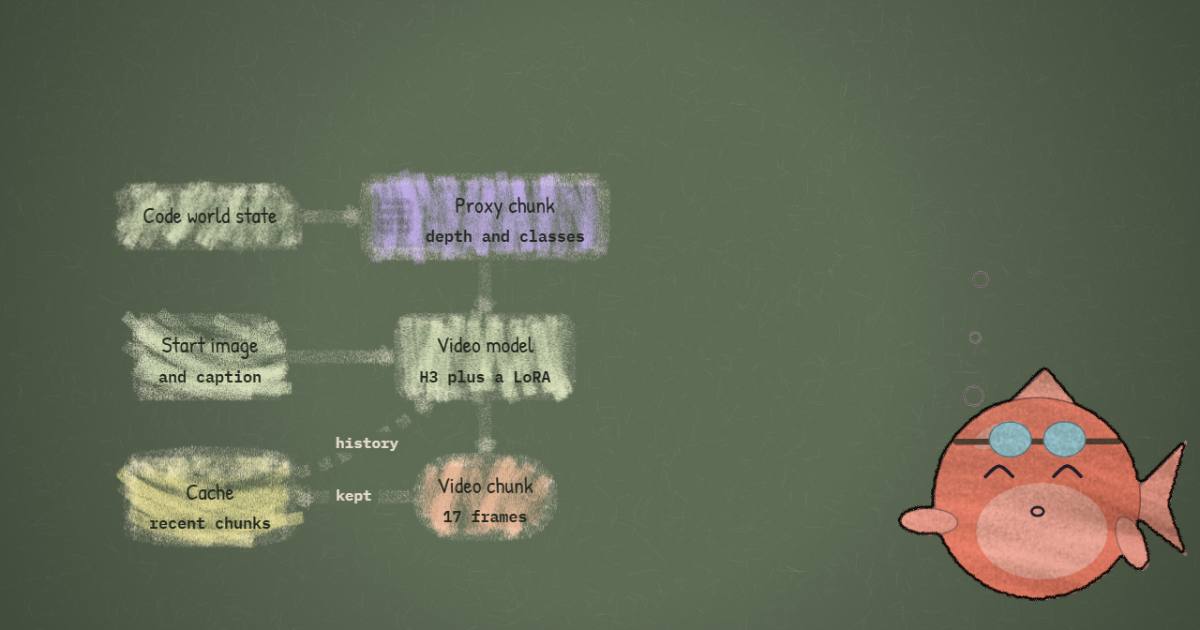
Now the clock. One chunk plays for 17/24 = 0.708 seconds. Rendering it takes 5.1, so the model produces video 7.2 times slower than real time, or about 8.3 seconds of video per wall-clock minute. The 60-second open-world streams in the post are 85 chunks, about 7.2 minutes of H200 time each.
And the 5.1 seconds is not the whole bill. In rtcwm/eval/evaluate.py, the per-chunk seconds come from the sampler's on_chunk callback, which brackets loading the span's inputs and running the transformer. The VAE decode happens after the whole stream is generated (evaluate.py:95), once, outside the timing. A live system would have to decode each chunk as it lands, so the real per-chunk cost is 5.1 seconds plus a decode that nobody has measured here.
To see what that means for a game, imagine one that produces proxy frames at 24 fps and hands each completed 17-frame chunk to one GPU. The first chunk can't start until its last proxy frame exists, 16/24 seconds in; its pixels exist 5.1 seconds after that, 5.77 seconds after the player did something. Every later chunk waits behind the one before, so the lag grows by 5.1 − 0.708 = 4.39 seconds per chunk. After a minute of play, the newest chunk on screen is more than six minutes old.
So the honest description is "causal, ready for a live proxy once the renderer is 7.2 times faster". Or a game whose clock runs at a seventh of real time, which for some uses (a turn-based world, a cutscene generator, a dataset factory) is fine. The README's own "(not yet real time)" is the right summary. The X post's "live proxy" is accurate about information flow and easy to misread about latency.
For scale, StreamRender-H3, the same backbone post-trained by NVIDIA, reports about 273 ms per chunk on eight GB200s with two denoising steps at 832x480. The comparison isn't like for like: different resolution, eight GPUs against one, a semantic map instead of depth plus semantics. It does show where the remaining factor of seven is likely to come from: fewer steps, lower resolution, more GPUs, and a sparser attention.
Memory: why this needs an H200
The README states 123 GB peak in bf16 and 108 GB with --fp8, and that "80 GB GPUs are not supported yet". That's a step backwards from CWM, which was tested on one 80 GB H800, but there it swapped 48 of the 50 blocks to host memory (blocks_to_swap: 48 in its tested settings), which is fine when you're rendering offline and fatal when you're streaming.
The checkpoint headers explain most of the rest. I read both safetensors headers by HTTP range request: each file holds 600 BF16 tensors, rank-128 LoRA pairs on 200 linears (the QKV, output and two MLP projections of 50 blocks), 596,377,800 parameters, 1.19 GB. CWM's LoRA has the same shape, so either file is a drop-in replacement on the same base. The QKV projection's output is 21,504 wide, three times 7,168, so each block's keys and values are 7,168 wide.
That gives the cache size. A chunk is 5 latents of 1,008 packed rows each, 5,040 rows. Keys and values for 50 blocks in bf16 come to 2 × 50 × 5,040 × 7,168 × 2 bytes, about 7.23 GB per chunk. Five chunks of history is 36.1 GB. Add the H3 transformer's weights, about 66 GB in bf16 for 33B parameters, and you are past 100 GB before activations, the condition rows, or the VAE. The 123 GB peak is about what the shapes predict. Getting this onto an 80 GB card means shrinking the cache (shorter span, quantized keys) as much as the weights.
Running it, and what it cost to train
This is a research release, not a package. You need the CWM release with its patched musubi-tuner, the MiniMax H3 weights, FlashAttention-3, an H200, and Slurm: every entry point is an sbatch script that assumes 8-GPU nodes. To regenerate data you also need CARLA 0.9.15, the open-code-world-model compiler and Qwen3-VL-32B for captions. The sampling commands from the README are short:
hf download Luffuly/streaming-code-world-model --local-dir ckpt

EVAL_ARGS="--steps 4 --rule x0 --shift 5 --kv-reuse" \
sbatch scripts/eval/eval.sbatch ckpt/streaming_dmd_4step.safetensors out/ clip_0048 clip_0244- safetensors
- 2 shards
- largest file
- 1.19 GB
- files
- 4
- downloads
- 0
- likes
- 2
repo last modified 2026-10-11
Licensing is the part to check before you build on it. The streaming repository has no licence file and the Hugging Face card declares none, so by default nothing is granted. CWM's own code is Apache-2.0. And the base model's licence is MiniMax's, which this site covered in the MiniMax H3 teardown: it excludes the US, UK, EU and South Korea.
Someone in the replies asked how many GPU hours training took. The README gives enough to estimate it: diffusion forcing on 8 nodes for about 7 hours is about 448 GPU-hours, and distillation on 4 nodes for about 5 hours is about 160 more, so roughly 600 H200-class GPU-hours for the two stages, before data rendering and pre-encoding. One inconsistency: scripts/train/distill.sbatch asks for 8 nodes, not the 4 the README mentions, so the distillation figure could be double.
What I'd take from it
The causal machinery is the reusable part. If you want to turn any windowed, bidirectional video model with rotary time positions into a streaming one, this repo is a compact, well-commented reference for the parts that are easy to get wrong: chunk on the VAE's own clip boundary, keep positions inside the trained range by counting from the span start, move cached keys with a rotation instead of recomputing them, make the text encoder causal too, and never train on clean history. The rtcwm package is about 3,200 lines of Python, and its docstrings explain decisions rather than restating code.
The world-model claim is still mostly CWM's, not this repo's. Streaming makes the code-plus-renderer split usable in a loop, in principle. Whether the coding agent can keep a world consistent for minutes, and whether a 3.54-second visual memory is enough once it does, needs a test where the camera comes back to something it saw a minute ago. The open-world clips don't do that, and the CARLA metric can't.
If you are comparing approaches, the useful neighbours on this site are StreamRender-H3 for the same backbone made fast with a simpler control signal, FastH3 for a 4-step H3 distillation aimed at speed, LongLive-Plug for distilled few-step adapters that transfer across H3 fine-tunes, and ABot-World-0 for a chunked autoregressive world model built for efficiency from the start.
How I checked
I cloned TingtingLiao/streaming-code-world-model at commit 64c489a and buaacyw/code-world-model at 17fa82b with git clone --depth 1 and read both; every file:line above refers to those commits. I did not run any of the code. I read the Code World Model paper on arXiv (2608.25927v1) and took its figures from the arXiv HTML. The cwm-proxy (open-code-world-model) repository asked for authentication, so I couldn't read it; what I say about it comes from rtcwm/data/proxy.py, which imports it.
The checkpoint facts come from the two safetensors headers on Hugging Face, read with HTTP range requests (no weights downloaded): tensor count, dtypes, shapes, LoRA rank and the metadata fields step: 1118, iter: 100 and objective. The KV-cache size is my arithmetic from those shapes and layout.py's 1,008 rows per latent frame; it assumes keys and values are cached in bf16, which is what the sampler stores. The H3 weight size is the 33B figure from this site's earlier teardowns.
The MSE, timing and memory numbers are the README's and the model card's, and I couldn't reproduce any of them without an H200. The real-time factor, drift ratios, lag model and GPU-hour estimate are my arithmetic on those numbers. The lag model is deliberately simple: one GPU, chunks back to back, no decode time, no frame dropping.