StreamRender-H3: the engine paints flat colours, a 33B video model paints the rest

mdjsonmcpcopy↗ai

2026-10-12 · 27 min · video-generation · world-models · distillation · kv-cache · realtime · diffusion

Why read this

Notable· top 60%

Rebuilds StreamRender-H3's chunk clock from its code: 273 ms per chunk is throughput; the shipped server shows a frame about 1.5 s after the engine drew it.

• Original analysis
• A new technique
• Concrete numbers to act on

·Image & video generation·Needs datacenter GPUs·Mixed licences·Practitioner model

How this was scored

Is it new?

2 of 3: A real new idea, method or capability

Can I trust it?

2 of 3: Measures key facts from files, code or configs

Can I run it?

1 of 3: API-only, gated or restrictive licence

Will I understand it?

2 of 3: Mechanism from first principles with figures

Can I act on it?

2 of 3: A concrete recipe, numbers or comparison

Will it last?

1 of 3: Relevant for months

Does it affect many?

1 of 3: A specialist community

Only here?

2 of 3: A teardown or measurement few others did

Score 60 of 100, ranked 267 of 494 rated articles. Each question is answered 0–3 by hand, and a 3 is rare. How articles are scored

I opened StreamRender-H3 expecting another world model: a network that is told "steer left" and has to imagine what the track looks like afterwards. Enze Xie's announcement reads that way. "Code drives the world. A game engine handles physics, object states, and player interactions, while H3 generates the visuals." Then "2 denoising steps, 24 FPS, and ~273 ms per chunk on 8×GB200 GPUs."

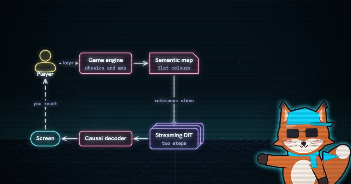
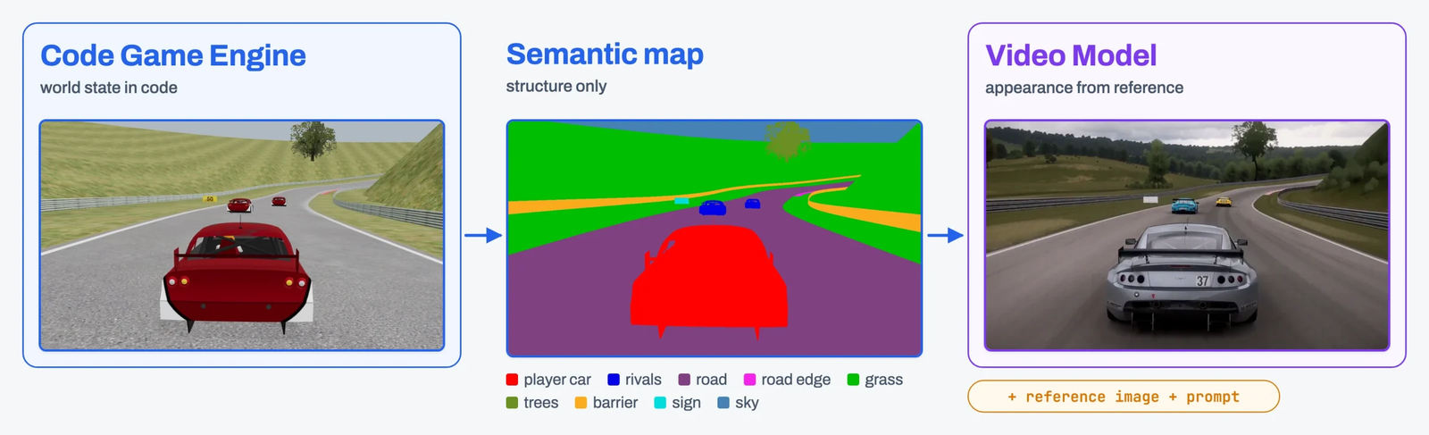
It is a more modest system than a world model, and I think a more useful one. The game engine never stops being a game engine. It keeps the map, the physics and the cars, and every frame it draws the scene with one flat colour per object class. The video model's only job is to paint over that colouring. It never decides where a car goes. It decides what the car looks like.

The code is public on the sol-engine branch of NVlabs/Sana, and so are the weights. So I read the runtime and the vendored H3 training code, pulled the safetensors headers, and checked the numbers on the project page against the files. Two things surprised me. The player's keystrokes never reach the model at all. And the 273 ms is a throughput number, a long way from how quickly a steering input shows up on screen.

What crosses the wire

The interface between the two halves is narrower than I expected. I went looking for G-buffers, depth, motion vectors, normals. There are none.

The engine is a three.js port of the TORCS E-Track 3 circuit and car (coding/threejs-racing/). Its SemanticView class (src/semantic.js) swaps every mesh's material for a flat ShaderMaterial whose fragment shader writes a single RGB constant, with tone mapping, fog, antialiasing and blending all off. The constants come from public/palette.json: 14 entries, 13 classes plus black for "unlabeled". Road is (128, 64, 128), the player's car is pure red, rivals are (0, 0, 230). Every frame becomes a 1344×768 PNG and goes to the GPU worker over HTTP. The worker decodes it and shrinks it to 832×480 with mode="nearest", with a comment saying why: "Semantic palette labels must not be bilinearly blended" (runtime/worker.py:96). A blended pixel between road and grass would be a colour that means nothing.

expand

The part I had to read twice is in the same file. The browser sends each frame with an X-Controls header carrying the keys held down. The worker writes those controls to controls.jsonl next to the timings (worker.py:110-114) and does nothing else with them. They are a transcript. If you brake, the engine's physics slows the car, the next semantic frames show the road scrolling slower, and that is the only way the renderer finds out.

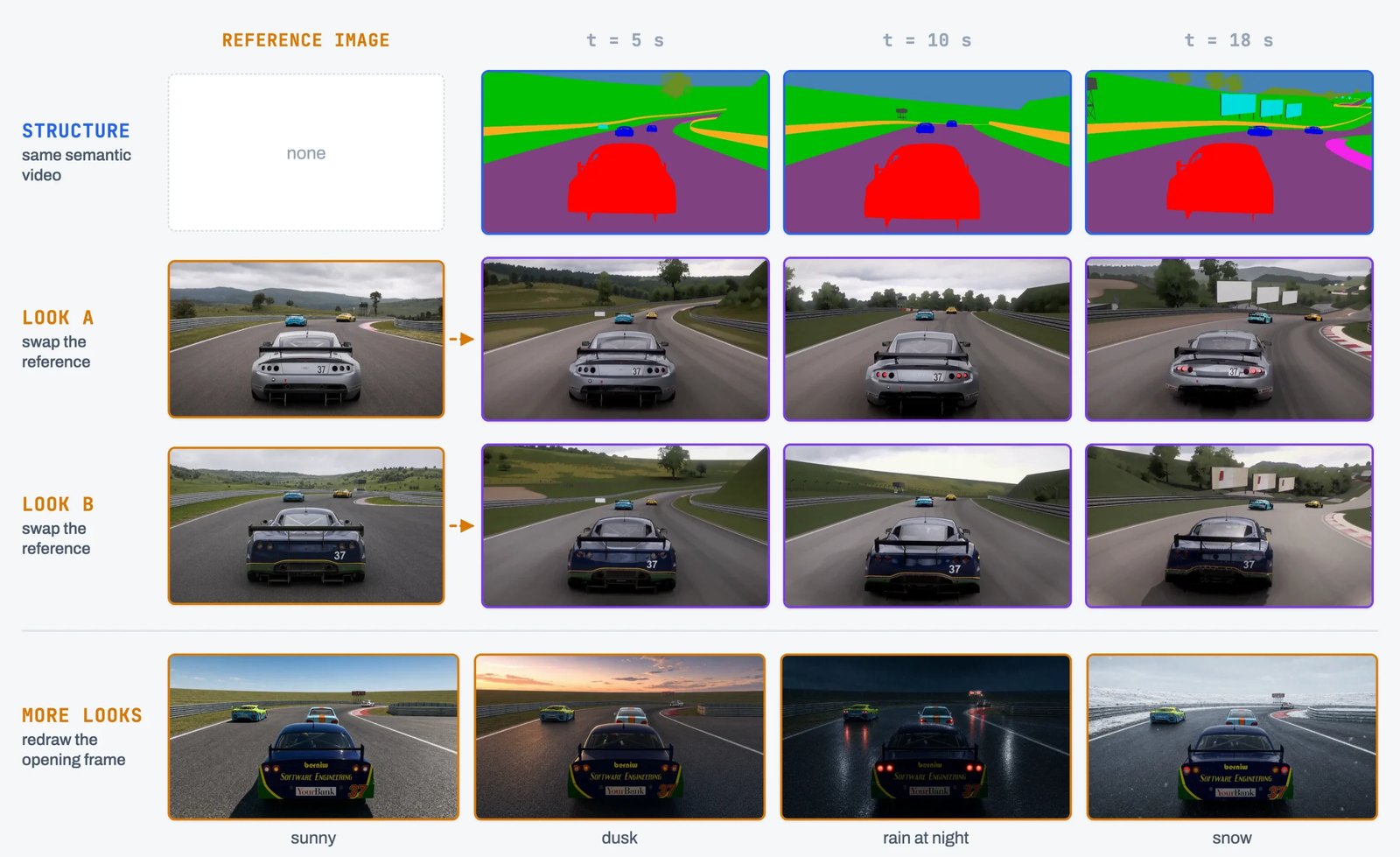
The project page wants it this way and says so: the semantic map should carry "everything that the world logic decides" and "nothing about how objects look". It also means the model cannot invent a consequence. A collision happens in the physics or it does not happen. NVIDIA's own DLSS 5 neural rendering is the obvious comparison, and the page draws it: DLSS 5 takes the colour and motion vectors of a frame the engine already rendered and re-lights it, so the engine still owns the look. StreamRender-H3 throws the engine's look away entirely and keeps only class labels, which is why a reference image can turn the same drive into snow.

H3 already had the right slot

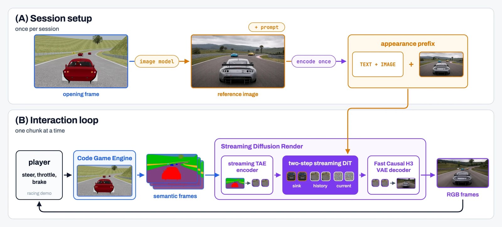
MiniMax H3 is the 33B video-and-audio transformer this site has taken apart for 8 GB cards and for four-step sampling. Its Ref2VA variant generates video and audio from a prompt plus reference images and reference videos. That last input is the trick. The semantic stream goes in as a reference video, and each of its latent frames lines up with the output latent frame at the same time step, so the layout of every generated frame is pinned to the map.

I counted the backbone in the released bundle: 535 tensors across nine safetensors shards, 33,122,992,912 parameters, all but 17.2M of them BF16. The full 50-layer H3, nothing pruned, with a LoRA merged in. The runtime refuses to start otherwise: if len(models["backbone"].dit.blocks) != 50: raise (worker.py:39-40).

The look comes from two inputs fixed for the whole session. An image model redraws the engine's opening frame as a photoreal screenshot with the same camera and the same cars, and a prompt in H3's structured template says which colour in the semantic video is which class and which input controls which property. A Qwen3-VL model (64 layers, hidden size 5120 in its config) reads the prompt and that picture once, at session start, and the result is cached. Swap the picture and the prompt, and the same semantic stream renders as another place.

expand

expand

The vendored code shows they tried other ways in. Next to the deployed meta-model sit classes that feed the semantic latents as the starting point of the noisy chunk (an SDEdit-style bridge at source_sigma: 0.95), concatenate them channel-wise onto the noisy video (24 + 24 input channels), and condition each token on backward optical flow through AdaLN. The deployed config uses none of them. It keeps the plain reference-rows path, MiniMaxH3VideoRefStreamingPrefixDMD with separate_reference_rope: true, which is the slot H3 shipped with. I can't tell from the code why the others lost; the page doesn't discuss them.

A window that slides, and a prefix that doesn't

H3 Ref2VA generates a whole clip at once with bidirectional attention. A game can't wait for the whole clip. StreamRender-H3 cuts the stream into chunks and denoises each chunk inside a window with two kinds of context, the design it credits to LynnReal-Omni: a sink (the opening of the stream, kept forever, in the spirit of StreamingLLM's attention sink and LongLive's frame sink) and the recent history.

The units are odd, and they matter for latency later. H3's video codec maps 17 RGB frames to 5 latents: the first latent of every five covers one frame, the other four cover four frames each. With merge_single_frame_units: true, the scheduler glues that one-frame latent to its neighbour, so units span 2, 1, 1, 1 latents and repeat. The shipped config is sink_size: 2, window_size: 2, chunk_size: 2, bootstrap_size: 7:

"chunk_size": 2, "sink_size": 2, "window_size": 2, "bootstrap_size": 7,
"merge_single_frame_units": true, "fps": 24, "height": 768, "width": 1344

Worked through, the first window generates 7 units, which is 9 latents, which is 30 frames. After that each chunk is two units, and because of the 2, 1, 1, 1 rhythm the chunks alternate between three latents (9 frames, 375 ms of video) and two latents (8 frames, 333 ms). Seventeen frames every two chunks, about 354 ms of video per chunk on average. Each current latent frame at 1344×768 is 1,008 tokens after the VAE's 16× downsampling and H3's 2×2 patches.

expand

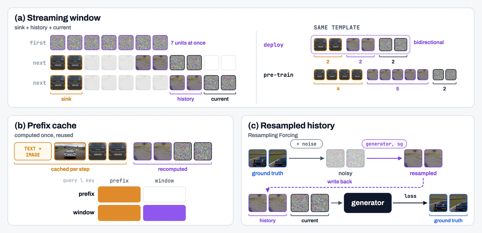
The window would be expensive if everything in it were recomputed every chunk. After the first continuation, the text and image conditioning, the reference picture and the sink never change, so the code splits the window into a fixed prefix and a moving part and gives them an asymmetric mask: the prefix attends only to itself, the moving rows attend to everything. That makes the prefix's keys and values a pure function of the session. They are computed once per denoising step and reused for every later chunk. The docstring in streaming_prefix_inference.py is precise about the granularity: "Each student, guidance branch and paired denoising time has its own prefix KV bank." Text rows carry the current video timestep, so the two steps can't share a bank.

The training stage that produces the deployed weights uses the same mask and recomputes the prefix with the current weights each step, so the model is trained on exactly the computation it runs at inference. Pre-training used dense attention and a wider window, four sink units and five history units, which the shipped config still records under teacher_streaming.

Three stages of training, none of them on real video

The training data surprised me more than the architecture. For the racing demo there are 10,000 paired clips of about 15 seconds, cut from about 5,100 recorded races on 39 tracks, every car driven by an AI driver. For each clip the engine records its normal render and its semantic video. An image-editing model the page names as GPT-Image-2.5 redraws the first frame as a photoreal screenshot, in one of ten lighting looks assigned in turn, 1,000 clips each. An LLM agent (Claude Opus 5.5) writes the prompts. And the photoreal target video is generated by native H3 Ref2VA at 25 denoising steps, in three five-second segments because the page found that after about five seconds the native model "no longer follows the semantic video and the reference image closely".

So the renderer learns to imitate H3's own output on synthetic pairs. The ceiling on how real it looks is H3 Ref2VA's, and the gain is speed and streaming, which is honest and what the page claims. Nobody should read the demo as a model that learned photorealism from racing footage.

Stage one is teacher forcing: one window per clip, history taken from ground truth. Stage two is Resampling Forcing, borrowed only for its resampling. Each training stream draws a noise level once, and at every window the ground-truth chunk is noised to that level and re-denoised by the generator without gradient before being written back as history. The current chunk is still trained against ground truth, but it now continues from context that contains the generator's own kind of mistake. Exposure bias is the usual way autoregressive video falls apart, and this fix is cheap because the generator does the resampling itself.

Guidance, folded into one call

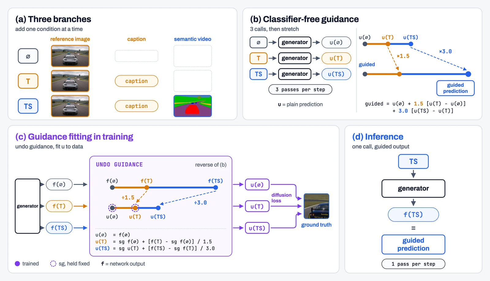
Following the semantic map closely needs guidance on the map, not only on the caption. H3 is guidance-distilled, so it samples with one forward per step; classifier-free guidance over caption and semantic video would take three. StreamRender-H3 trains the guidance into the weights instead, extending LynnReal-Omni's caption-only version to a chain of three branches: ∅ (reference image only), T (adds the caption) and TS (adds the semantic video). Guidance would stretch the caption step by 1.5 and the structure step by 3.0. Training runs that backwards. Treating each raw output $f$ as already guided, it undoes the stretches,

holds the lower branches with stop-gradients, and trains $u(TS)$ against the data with the ordinary diffusion loss. Once that converges, a single call of $f(TS)$ is the guided prediction.

Work the coefficients out and something tidy falls out, which the page writes but doesn't comment on: $u(TS) = \tfrac{1}{3}\big(f(TS) + f(T) + f(\varnothing)\big)$. At these two scales the quantity the loss sees is the plain average of the three branches. The general form, from the sequential-fitting section of minimax_h3/streaming_sft.md, is $f(TS)/s_1 + (1/s_0 - 1/s_1)\,f(T) + (1 - 1/s_0)\,f(\varnothing)$.

expand

Two steps, trained on its own rollouts

After guidance fitting the generator samples a chunk in 16 steps, which is far too slow. Stage three is distribution matching distillation (DMD, DMD2) on the generator's own rollouts, as in Self Forcing: each training step generates the current window of every stream from the generator's earlier output, computes the loss on that chunk only, and writes the chunk back. It runs on the first 30 seconds of 5,000 sixty-second drives, with no target video at all.

expand

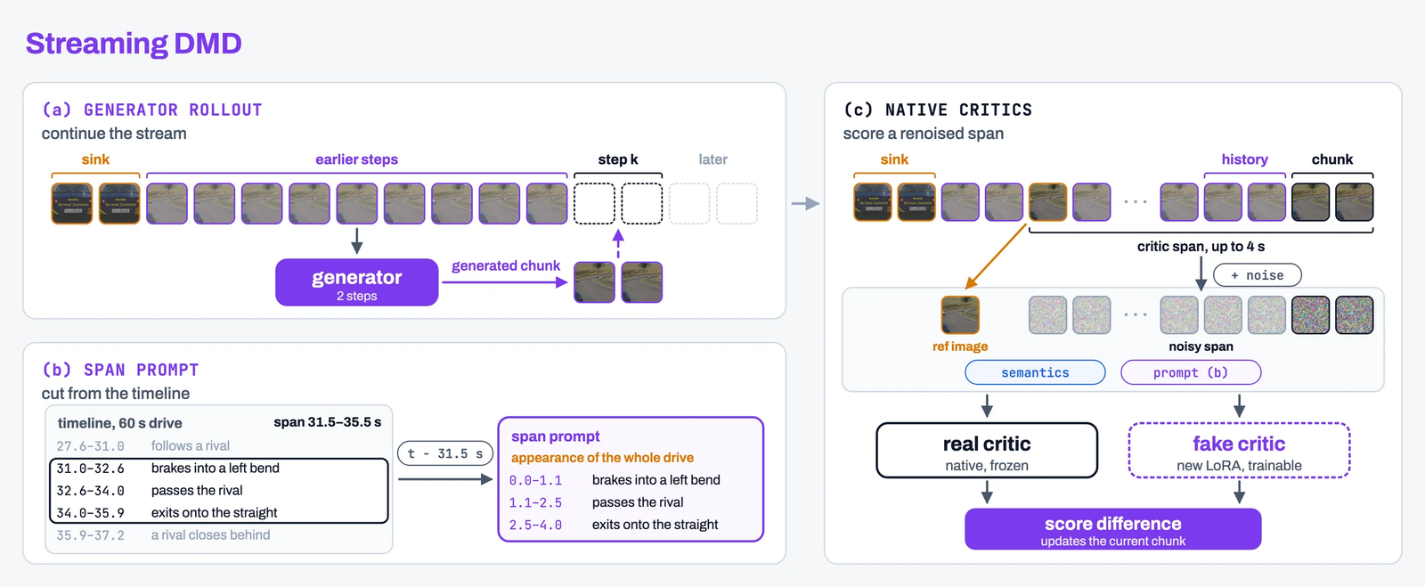
The critics are the clever part. Both are the native, bidirectional H3 Ref2VA, and each scores a span of up to 29 latent frames, about four seconds, ending at the current chunk, using the frame at the start of the span as its reference image. Native H3 is good for about five seconds before it drifts. Four-second spans keep the critics inside the range where they can be trusted. The cost is that a span needs its own prompt, and the page reports that without timestamped actions the model "sometimes even renders the semantic video in reverse". So every drive is labelled once by an agent (the page names GPT-6.1 Sol) with a timeline: phases of 2 to 10 seconds, events of 0.3 to 2.5 seconds, and a scene state every half second, cut and re-clocked for each span.

The checkpoint name in SOURCE_SNAPSHOT.json tells the same story in one line: 1008b_torcs_timeline_critic_native_dmd_s2w2c2_2step_30s_..._fake_cfgfit3_4, step 0000224. Timeline critic, native critics, S2/W2/C2, two steps, 30-second streams, a fake critic fitted at 3 and 4 (the page says the fake critic uses guidance fitting at 3.0 and 4.0). The released weights are step 224 of that DMD run. One small inconsistency: the shipped runtime.json still carries a cfg_fitting_guidance block with scales 1.5 and 3, which only matters during training, where the fake critic exists.

The decoder an agent built

The VAE is where most streaming video projects quietly give up quality, and StreamRender-H3's answer is the most interesting engineering story on the page.

H3's released decoder is a 36-layer, 2.42B-parameter transformer built for offline video. It splits a frame into overlapping 256-pixel tiles and decodes five latent frames together with the next two, so it both recomputes overlap and waits for latents that do not exist yet. The tiny streaming TAE decoder runs in about 10 ms but, in their runs, reached only 27 dB PSNR against the full VAE and made grass and road texture flicker.

They gave a coding agent (Claude Code) one goal and four constraints: strictly causal, two latent frames per call, within 50 ms per call at 720p, start from the released weights. The page walks the iterations in order. It pruned greedily to 24 of the 36 layers (kept: 0 to 17, 19 to 21, 31, 32, 35, which matches the keep_layers list in runtime.json). It replaced tiling with non-overlapping 16×16-token windows that shift by half every other layer, and replaced lookahead with a cache of the previous four latents' keys and values. I counted the shipped decoder: 1,617,806,936 parameters, all FP32, which is the 1.62B the page gives.

expand

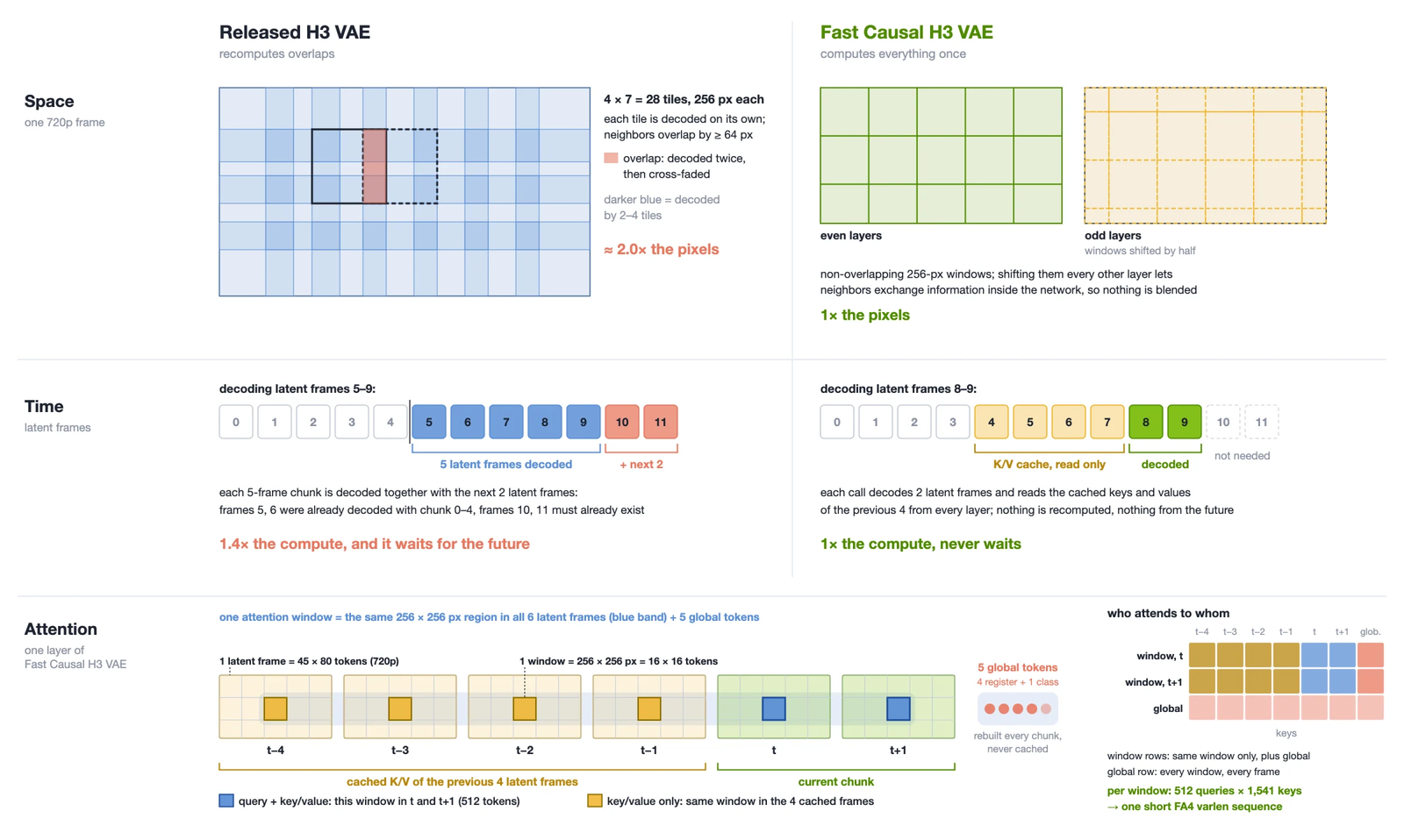
My favourite paragraph on the page is iteration 4, a bug the metrics missed. The decoder has four register tokens and a class token that attend to the whole frame. In the released decoder they carry no time position, which is harmless when every chunk is decoded from frame 0. The causal decoder can't renumber its frames, because cached keys keep the positions they were computed at, so frame tokens carry absolute stream time while the registers carried none. Trained on clips of ten latent frames, the decoder made the first frame of every five-latent block about 20 grey levels darker from the eleventh latent onward. Averaged PSNR didn't show it. Someone watching the stream did. Giving the registers the time position of their chunk makes every attention score depend only on time differences, and the code has it: _suffix_ids(self.t, ...) sets the suffix tokens' rotary position from the chunk's own time (causal_vit_stream.py:176). The result is reported as identical output whether the stream clock starts at 0, 100 or 1000.

After distillation and two optimisation loops (the second run by NVIDIA's Kernel Design Agents), the page reports 23.8 ms per two latent frames at 720p on one GB200, against 326 ms for the official decoder on the same call, with 33.04 dB PSNR against the H3 VAE (TAE: 27.11) and LPIPS 0.056 (TAE: 0.153).

expand

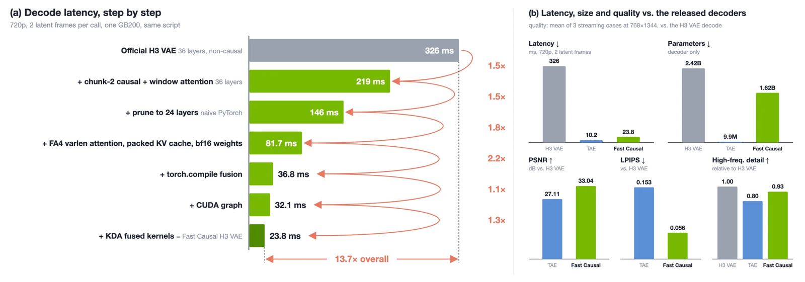
One property of this decoder matters for latency and isn't on the page. It decodes latents strictly in pairs at absolute indices 2k and 2k+1 (causal_vit_codec.py, "every 2 consecutive latents ... are decoded together as soon as both exist"). The DiT's chunks hold three latents, then two, then three. Whenever a chunk ends on an even index, that last latent's four frames sit in the decoder until the next chunk arrives.

Where the 799 ms went

The DiT step is the bulk of the time, and the page's ablation shows something I like seeing in a speedup story: one idea did most of the work. On eight GB200s with Ulysses-style sequence parallelism and a full copy of the weights per GPU, a PyTorch baseline took 799.66 ms per two-step chunk. Static-context KV caching, the prefix bank above, brought that to 315.42 ms on its own. Everything after it, AdaLN projection caching, a FlashAttention-4 kernel tuned for these shapes, attention metadata reuse and a persistent KV layout, took 315.42 to 217.96. Those are worth doing. They are also a third of the gain, and they ride on the Sol-Engine stack the SANA articles describe.

expand

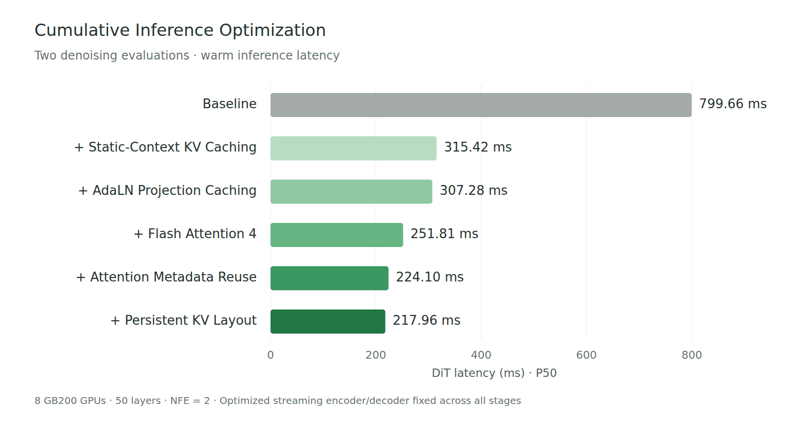
The AdaLN cache is the same observation FreeVideo made from the other direction: H3's AdaLN modulation depends only on the timestep, so with a fixed schedule it is a lookup table. Here it is guarded by exact tensor equality on the input (render/optimizations.py), so it can never return a stale projection.

Then the 273. The tweet says "~273 ms per chunk"; the page's headline says 218 ms. They are different measurements, and the page's own latency JSON says which is which. render_p50_ms is 217.96, the DiT alone. The encoder's p50 is 16.67 ms and the newer decoder is 23.8 ms. And original_run_rgb_ready_tpot_p50_ms is 272.73, the time from a chunk's input to its RGB being ready, measured in a run that still used the older 36.5 ms decoder. The JSON adds that the stage values "are not an additive newly measured end-to-end TPOT". So 273 ms is the honest end-to-end figure, a median, and slightly stale in the good direction.

expand

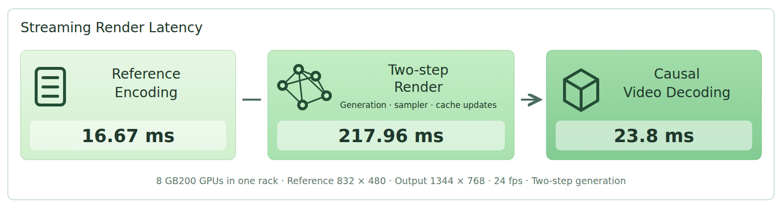
273 ms is how fast it keeps up, not how fast it answers

A chunk is about 354 ms of video, and the renderer needs about 273 ms to make one. So it keeps up with 24 fps with room to spare: the GPUs are busy about 77% of real time, and the capacity works out to roughly 31 frames per second. The claim holds.

Interaction latency is a different quantity, and the page never reports it. The code logs a per-chunk oldest_input_to_rgb_ready_ms (worker.py:106), but no value is published. So I rebuilt the schedule from the runtime's own rules and timed it.

Three rules set it. The worker calls session.collect(frames, ...) and does not start a chunk until every engine frame in it has arrived, so the first frame of a nine-frame chunk has waited 333 ms before the GPU starts. The decoder holds an unpaired latent until the next chunk. And the HTTP server paces output at 24 fps from the first frame it sends and never skips ahead:

# runtime/server.py, the stream loop
delay = deadline - time.monotonic()
if delay > 0:
    time.sleep(min(delay, 1 / 24))
...
deadline = max(deadline + 1 / 24, time.monotonic())

That last rule is the one with consequences. The first chunk is the 30-frame bootstrap, so the first rendered frame can't appear until the engine has drawn 30 frames (1.21 s at 24 fps) and the bootstrap has rendered. The playback clock starts there and then runs at exactly the engine's rate. Whatever lag the bootstrap created, every later frame inherits.

With 273 ms per chunk, and assuming the bootstrap costs the same as a normal chunk, every frame reaches the screen about 1.48 s after the engine drew it (1,481 ms in the simulation: the lag as shipped). The bootstrap is a bigger window with no prefix cache, so its real cost is probably higher, and every extra millisecond of it is added to the lag for the rest of the session; the page publishes no bootstrap timing. A server that re-synced once after the bootstrap, skipping ahead to live, could hold a fixed lag of about 0.77 s (773 ms), and about 0.61 s if the decoder did not wait for pairs. Below that you are fighting the chunk itself: a nine-frame chunk can't start until its ninth frame exists.

These are reasoned from the code with transport, PNG and JPEG encoding and the browser left out, so the real numbers are higher, not lower. For a third-person racing game, a lag of half a second or more is noticeable but drivable, the way cloud gaming on a bad connection is. For anything twitchier it would not be. A reply under the announcement asks whether the picture keeps up when the view turns quickly; it had no answer in the thread when I read it.

Two smaller things follow from the same arithmetic. The headroom is a median against a mean. The page's own decoder section reports DiT rounds of 264 to 329 ms in an earlier eight-GPU loop; at 329 ms, plus the 37 ms that loop's decoder took and the encoder's 17, a nine-frame chunk is over its 375 ms budget. One slow chunk is absorbed by the playback buffer. A sustained run of them grows the lag until the bounded 48-frame input queue fills, at which point the server returns 429 and the engine stops advancing its own clock. The runtime never drops a frame; it slows the game down instead. And the cost: one session per worker allocation, eight GB200s per player.

Can you run it

Yes, if you have the hardware and the right passport. The bundle at Efficient-Large-Model/StreamRender-H3 is 206.87 GB and holds every component: the merged backbone in nine shards (66.28 GB, reassembled by a script that checks its SHA-256), the causal decoder (6.47 GB, FP32), the Qwen3-VL conditioning model twice (safetensors and a DCP conversion), the TAE encoder, the H3 audio codec and the default reference image. The README calls for eight GPUs in one NVLink domain, and the worker accepts four or eight. The tested kernels are FlashAttention-4's CuTe backend, which targets Blackwell.

The licensing is mixed. The runtime code is Apache-2.0. The renderer, decoder and audio codec are H3 derivatives under the MiniMax H3 Community License, whose "Excluded Territories" are the European Union, the United Kingdom, the Republic of Korea and the United States. Qwen keeps Apache-2.0 and the TAE keeps MIT.

There is no paper. The project page is a research blog and asks to be cited as one, together with the Sol-Engine paper, which covers the inference stack, not the renderer. And there is one scenario: everything, including the critics, is trained on the racing game with a chase camera. The page says so plainly and lists more games as the next step. Asked whether eight GB200s is a starter setup, Xie replied that it "ideally should run this on RTX series GPU". A hope, then, not a release.

What I take from it

The split is the idea worth keeping. Let code own everything that has to be exact and repeatable, hand the model nothing but class labels, and the model can't break the game. It also can't improve it, and that's fine. The training recipe is careful in the places that usually fail: critics confined to the span where H3 is trustworthy, prompts cut to that span, a prefix cache that training sees too, and a decoder whose worst bug was caught by watching the video rather than the averages.

The latency story is where I'd push back. "24 FPS" and "~273 ms per chunk" are both true and both throughput. A player feels the other number, which the runtime is already logging, and which by my reading of its schedule is closer to a second and a half as shipped. The fixes are in the plumbing, a resync after the bootstrap and a decoder that doesn't hold half a pair, before anyone has to make the 33B model faster.

How I checked

I shallow-cloned NVlabs/Sana at the sol-engine branch and read models/streamrender_h3/ (runtime, engine, decoder, configs) and the vendored H3 code under render/vendor/ (the window planner in minimax_h3/data/streaming.py, the prefix-bank and prefix-DMD modules, both streaming_sft.md design notes, the timestep and sampler classes). I ran none of it. I read the project page, its latency JSON and the X thread and replies through the fxtwitter mirror. Parameter counts and dtypes come from the safetensors headers of the Hugging Face bundle, read with HTTP range requests; sizes and the licence from the repository's file listing, README, NOTICE and LICENSE. The latency figures are my simulation of the schedule the code implements (chunk boundaries from the unit rules, a render cost per chunk, pairwise decoding, the server's pacing rule); the interactive above runs the same model. Everything quoted from the page about training data, iterations and timings is the project's own report; I could not check any of it.

One thing I could not settle. The shipped runtime.json sets the timestep scale "T": 1 as an integer, and TrailingSamplingTimesteps rounds the grid to integers when T is not a float. Read literally, a two-step grid of 1.0 and about 0.86 (shift 6) becomes 1 and 1, and the second step would start from the same noise level as the first. The design notes write T: 1.0, and I may be missing a conversion somewhere, so I am not calling it a bug; but it is a five-minute check for anyone with the hardware, and it would decide whether the second of the two denoising evaluations is doing anything.