2026-10-08 · 26 min · transformers · pretraining · scaling-laws · positional-encoding
Why read this
Notabletop 60%LayerRoPE rebuilt from its equations; the 3.4x re-derived (1.6x vs the best baseline) and the rotation premise tested on LLaMA-2 weights.
- Original analysis
- A new technique
- Concrete numbers to act on
LLM architectureRuns on a consumer GPUResearch paper
How this was scored
- Is it new?
- 2 of 3: A real new idea, method or capability
- Can I trust it?
- 2 of 3: Measures key facts from files, code or configs
- Can I run it?
- 1 of 3: API-only, gated or restrictive licence
- Will I understand it?
- 2 of 3: Mechanism from first principles with figures
- Can I act on it?
- 2 of 3: A concrete recipe, numbers or comparison
- Will it last?
- 1 of 3: Relevant for months
- Does it affect many?
- 1 of 3: A specialist community
- Only here?
- 2 of 3: A teardown or measurement few others did
Score 59 of 100, ranked 264 of 476 rated articles. Each question is answered 0–3 by hand, and a 3 is rare. How articles are scored
A week ago I wrote up DepthBench, which found that a plain Pre-Norm Transformer gets worse as you trade width for depth, and that only the redesigned residual streams (Hyper-Connections, Attention Residuals) make extra layers pay. So when @arXivBangers posted a paper claiming a fix that touches nothing but the normalization weights, I wanted to know how a change that small could matter.
The paper is LayerRoPE (Shikhar Srivastava and Christopher Kanan, University of Rochester, 6 Oct 2026). Its pitch: the residual stream's growth with depth is not a disease, the norm weights of trained LLMs already encode which layer they sit in, and if you make that encoding explicit, with a magnitude and a rotation borrowed from RoPE, you get a model that reaches Pre-Norm's 1.3B loss with 3.4x less compute and still trains at 512 layers.
Two things surprised me. The method is tiny: per site, one shared gain vector and four scalars, sixteen scalars for the whole network. And the "RoPE" half of it, the rotation, turns out to be the weakest part of the evidence, both in the paper's own ablation and in the pretrained weights I read. The magnitude half holds up well. The headline 3.4x is real arithmetic on the paper's plot, but it is measured against the weakest baseline, at sequence length 256, on a recipe with no gradient clipping. There is no code yet; the project page linked from the paper returned a 404 when I checked.
Why depth is hard, in two equations
Every Transformer layer is a pair of sublayers (attention, then MLP), and the only question that matters for depth is where the normalization sits relative to the residual add.
Post-Norm, the original 2017 layout, normalizes after the add:
The stream never grows, because it is renormalized every layer. But the gradient has no clean path home: every layer's backward pass goes through a normalization Jacobian, and those products compound. Xiong et al. showed the gradients near the output are large at initialization, which is why Post-Norm needs a learning-rate warm-up and why it falls apart as you stack layers.
Pre-Norm moves the normalization inside the branch:
Now there is an identity path from the loss to every layer, so it trains at any depth. The cost shows up in the forward pass. Each block reads a normalized input, so its output has roughly fixed size no matter how big the stream has become, while the stream itself is a running sum that keeps growing. By layer a new write is one term against earlier ones, and its relative effect shrinks roughly like . Sun et al. named this the curse of depth: deep Pre-Norm layers end up close to identity maps, and you can delete many of them with little loss.
The fixes so far come in two families, and the paper frames itself against both.
The first damps something. DeepNet keeps Post-Norm but up-weights the residual by a constant and shrinks the initialization of some projections, which bounds each update and got a 1,000-layer model to train. Layer-Norm Scaling (Sun et al.) multiplies each block's normalized input by . Peri-Norm, which Gemma 2 ships, normalizes both the input and the output of every block. ReZero and LayerScale gate each branch with a learned scalar that starts near zero. Mix-LN uses Post-Norm in early layers and Pre-Norm in later ones; LayerRoPE does not cite or compare against it, which is a gap.
The second family rebuilds the residual path itself. Hyper-Connections widen the single stream into several (see xHC for the current state of that line), and Kimi K3's Attention Residuals replace the uniform sum with a learned read over earlier layers.
LayerRoPE's position is the contrarian one. It does not try to keep the stream small; its learned model ends up with a bigger stream than Pre-Norm's. What it controls is how much each block reads from the stream and how much it writes back, as a function of depth.
What trained models already do with their norm weights
The paper starts from an observation. In a Pre-Norm model, the RMSNorm weight is the one learned per-layer gain that sits directly on the path from the stream into each block. If the network wanted a per-layer dial, that is where it would put it. Across 16 open models from 9 families, the authors look at those vectors and report two patterns: their magnitude grows with depth, and their direction rotates.
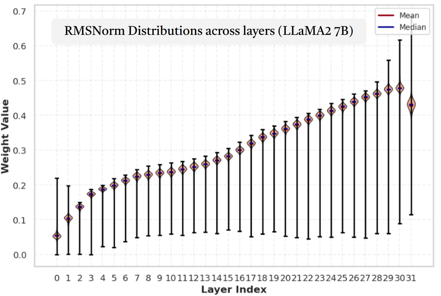
The magnitude part I could check directly. I pulled the 64 RMSNorm weight vectors of LLaMA-2 7B out of its safetensors with HTTP range requests, about 8 KB each, without downloading the model. The paper's plot starts at a layer-0 mean of 0.055; mine does too. The root-mean-square of the MLP-input gain grows from 0.056 at layer 0 to 0.478 at layer 30, and a power law fits it with in log space. That matters because a power law in is exactly the form LayerRoPE builds in. On this one model, the magnitude premise holds up.
The rotation part is where I disagree with the paper's reading.
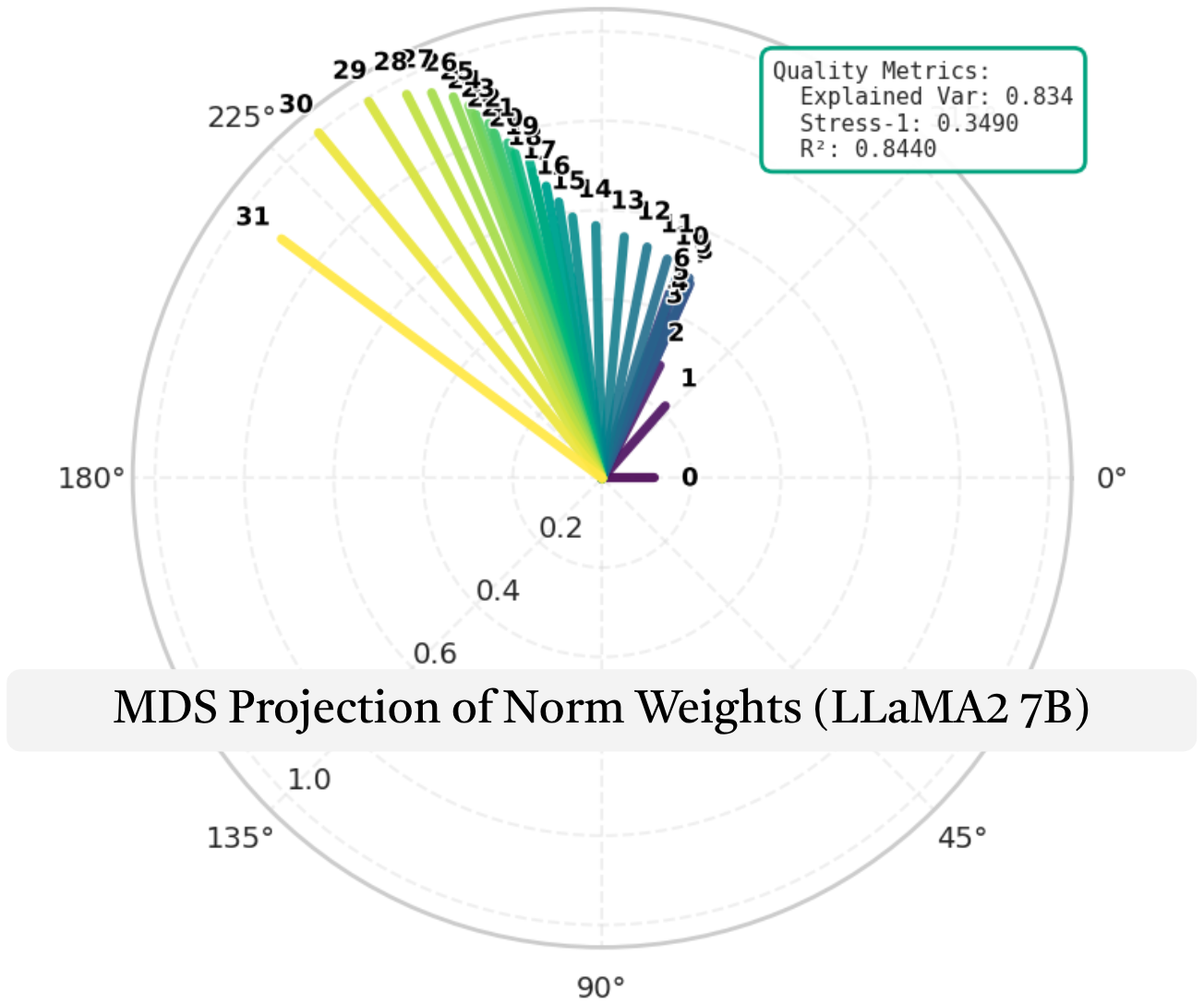
That angle is measured inside a two-dimensional MDS embedding, not between the vectors themselves, and the paper does not say what point the angles are taken around. The plot's own quality box reports a stress of 0.349, which by the usual rule of thumb is a poor fit. So I measured the angle in the space the vectors live in, :
- Between any two layers' MLP-input gains, the largest angle is 12.3 degrees.
- The single step from layer 0 to layer 1 accounts for 11.0 degrees of it.
- From layer 1 to layer 31 the direction moves 7.7 degrees while the norm grows 4.2x.
The MDS angle has a simpler explanation. I generated 32 copies of one fixed vector, scaled from 1 to 8 with 5% noise, whose true pairwise angles never exceed 4.2 degrees. Projected the same way and read around the centroid, that pure-scaling control sweeps 176 degrees, because a line of points seen from its own middle spans half a turn. A large swept angle in an MDS plane can be produced by a vector that only grows.
The paper's own Appendix C says much the same in other words: about 99% of the dimensions follow one shared magnitude trajectory, and the "rotation" comes from about 1% of outlier channels. My numbers agree with that decomposition. Where I disagree is the framing that comes after it. In LLaMA-2, direction is a small, early-layer effect, and magnitude is most of what changes. Keep that in mind when you get to the ablation.
The construction: RoPE's polar form, applied to a gain vector
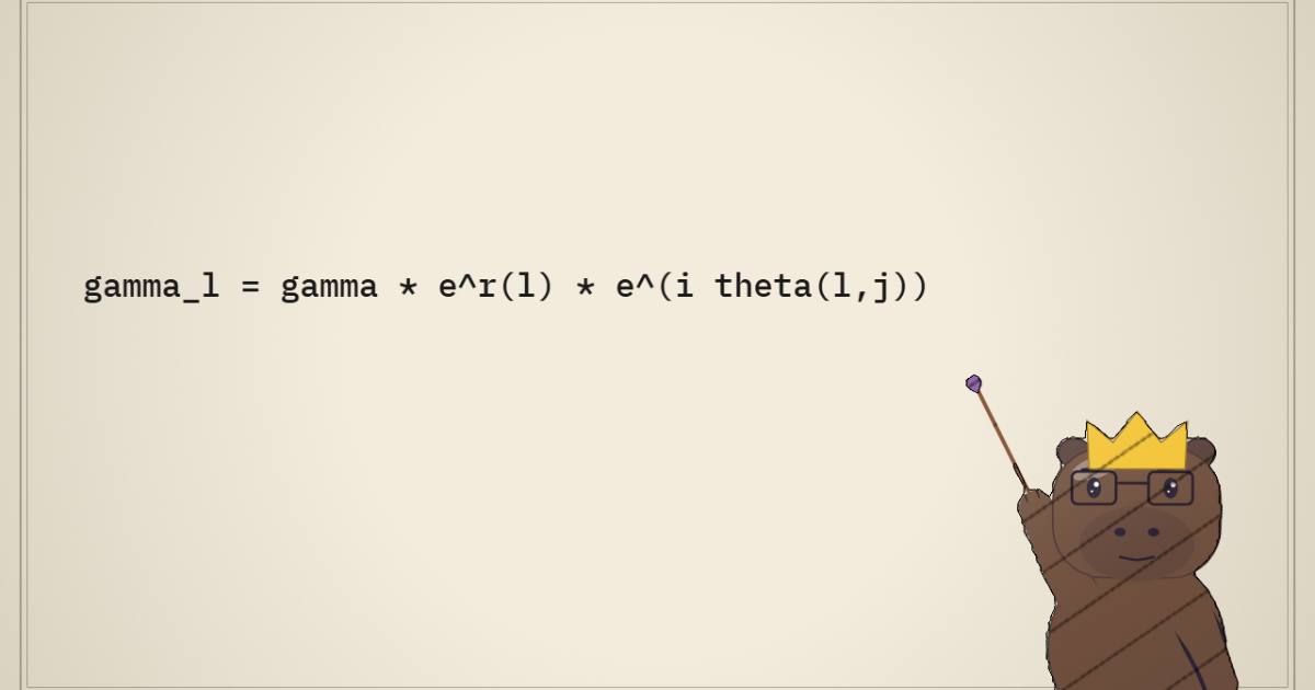
RoPE (see the RoPE explainer) treats a query or key as complex numbers and multiplies pair by , where is the token position and is a geometric spectrum of frequencies. LayerRoPE borrows the same polar form and points it at a different object and a different index: the norm gain instead of the activations, and the layer index instead of the token position.
Here is one shared vector per site, read as complex pairs , and multiplies pair by pair. There are four sites per layer: the read into attention, the write out of attention, the read into the MLP, the write out of the MLP. The two schedules are:
Exponentiate them and both are power laws in depth. The magnitude multiplier is , the same shape as Layer-Norm Scaling's but with a learned slope and offset. The base angle is , spread over the channel pairs with base , so the first pair turns by the full angle and the last by about a hundredth of it. Both slopes start at .
The "superposition" in the title is this polar form: a complex number's modulus and phase, multiplied together. A rotation leaves each pair's modulus alone, so exactly. The magnitude schedule sets the length of the gain vector and the rotation sets only its direction.
The analogy to RoPE stops at the arithmetic. RoPE works because the rotated vectors meet in a dot product: depends only on , which is what makes it a relative position code. Nothing here takes a dot product between layers. The rotated gain is just a per-channel scale applied elementwise to . Write out what rotating one pair does to the two gains it holds:
If the shared gain starts at all-ones, as RMSNorm weights usually do (the paper does not print its learned ), pair becomes . So rotation moves gain from one channel of a pair to its neighbour, by an amount that depends on depth and on the pair's frequency. Past 45 degrees the first channel's gain goes negative. It is a legitimate way to give each layer a different per-channel weighting with almost no parameters. I would not call it a positional encoding in RoPE's sense, though. The name oversells the mechanism a little.
The widget builds one layer's gain from the paper's learned 1.3B values. The slopes are printed in its Figures 20 and 21; the layer-0 values I read off those plots. On the right is the LLaMA-2 measurement from above.
Each dial is one channel pair of the shared gain, drawn from all-ones (dashed). LayerRoPE scales every pair by the same er(l) and rotates pair j by θ(l)·100−2j/d, so the first pair turns by the full base angle and the last by about a hundredth of it. Rotating (1, 1) moves gain from one channel of the pair to the other; past 45° the first channel's gain goes negative. Slopes are the paper's learned 1.3B values (Figures 20 and 21); layer-0 values are read off those plots.
Two things stood out while I was building it. The learned base angles all decay hard with depth: at the MLP read, the slope is , so a base angle near 49 degrees at layer 0 is down to about 1.5 degrees by layer 23. Averaged over all 1,024 pairs of a 2,048-wide gain, the whole vector turns about 16 degrees at layer 0 and about half a degree at layer 23. The LLaMA-2 measurement has the same shape: nearly all the turning happens at the bottom of the stack. Trained with the rotation available, the model chose to use it mostly in the first few layers.
The parameter arithmetic also checks out. Pre-Norm has gain parameters (two norms per layer); LayerRoPE has four shared vectors plus sixteen scalars, . At the 1B tier (, ) that is fewer, exactly the 90.096K in the paper's Table 5. The FLOP overhead is the new write gate, per training token, which is 0.0051% of the 7.72 GFLOPs per token at 1B and 0.0128% at 60M. It is effectively free.
The method is short enough to write out. This is my numpy reading of the equations, not the authors' code, which is not public. It builds all gains for one site:
# layerrope_gain.py, my implementation of the paper's Eq. 1 (not the authors' code)
import numpy as np

def layerrope_gains(gamma, L, a_mag, b_mag, a_rot, b_rot, base=100.0):
    """All L per-layer gains for one site, from one shared gamma (shape [d])."""
    d = gamma.shape[0]
    l = np.arange(L)[:, None]                                  # [L, 1]
    r = a_mag + b_mag * np.log(l + 1)                          # magnitude, log-linear in depth
    theta = np.exp(a_rot + b_rot * np.log(l + 1))              # base angle per layer
    theta = theta * base ** (-2 * np.arange(d // 2) / d)       # RoPE spectrum over pairs, [L, d/2]
    g = gamma[0::2] + 1j * gamma[1::2]                         # read gamma as d/2 complex pairs
    g = g * np.exp(r) * np.exp(1j * theta)                     # scale and rotate
    out = np.empty((L, d))
    out[:, 0::2], out[:, 1::2] = g.real, g.imag
    return out                                                 # [L, d]: use row l as layer l's norm weight
With gamma = ones(2048), both offsets at zero and both slopes at , the row norms come out at exactly , and 54 channels of layer 0 have negative gain. Because the gains depend only on , a framework computes them once per step and broadcasts; the gradient flows into five tensors per site instead of .
Read less, write more
The idea that carries the paper is easier to see in its overview figure than in the equations.
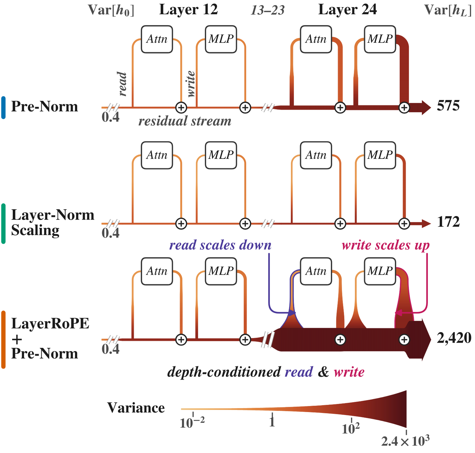
In a Pre-Norm backbone LayerRoPE does two different things. At the read sites it replaces the existing RMSNorm weight, so it can turn a block's input down with depth, as Layer-Norm Scaling does with a fixed . At the write sites it adds something Pre-Norm does not have at all: a per-channel gate on every sublayer output, before the residual add. Both slopes start at . The learned model takes them to opposite signs.
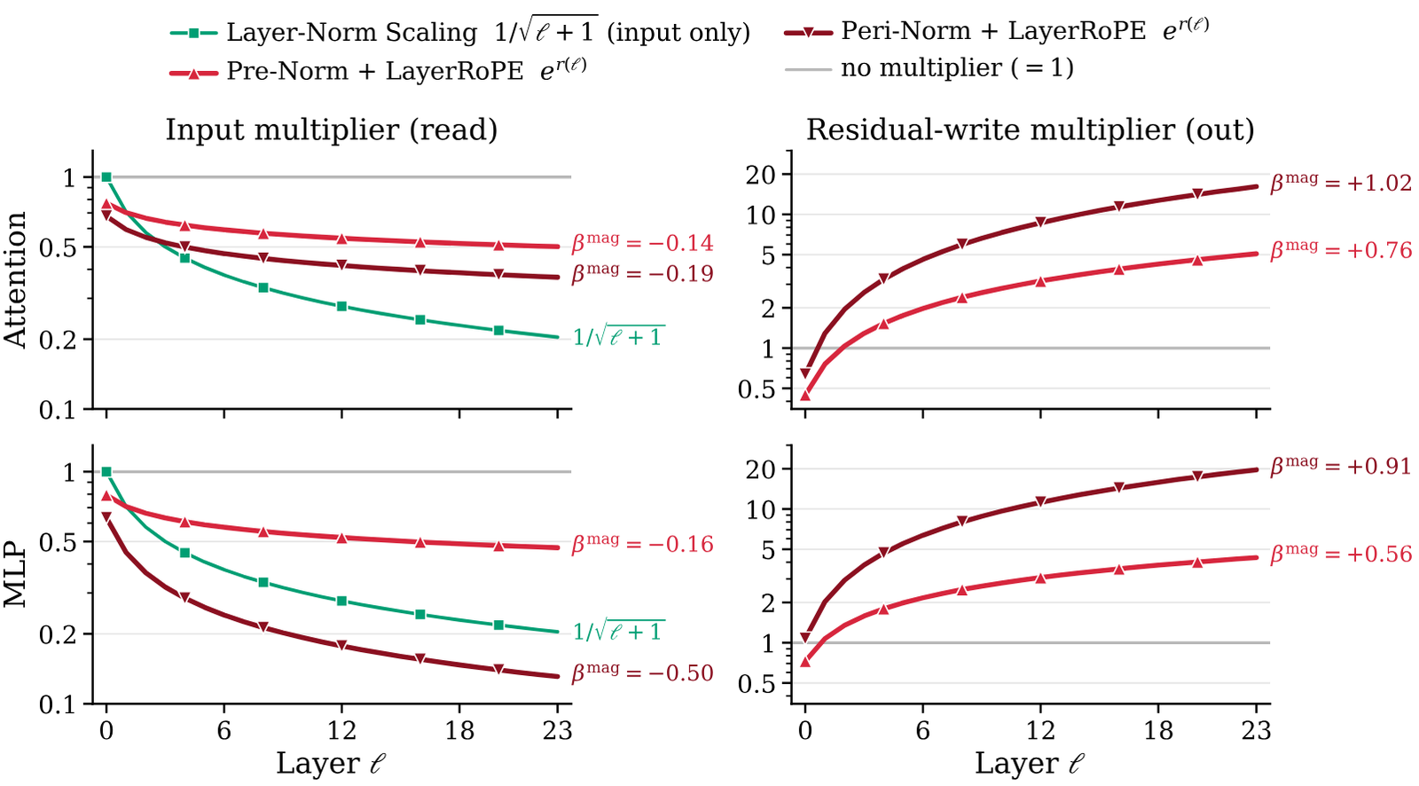
The write slopes go from to and on the Pre-Norm backbone and to about on the Peri-Norm one. The paper's Figure 22 adds an interesting detail. Layer-Norm Scaling's own free per-layer norm weights learn to undo most of its prescribed , never letting the effective attention-input ratio fall below about 0.75. The optimizer, given the freedom, does not want the reads damped as hard as LNS damps them, and it does want the writes louder.
Why would bigger writes help? Go back to the dilution argument. If every layer writes a fixed-size update into a growing sum, late layers are whispering into a crowd. A write gain that grows with depth lets them keep up. The widget below is a toy that isolates exactly that and nothing else: each block is held at unit gain, its write is assumed independent of the stream, and only the depth schedule changes.
A toy, not a measurement. Each block is held at unit gain and its write is assumed independent of the stream, so the only thing that changes between lines is the depth schedule on the read and write gains. The learned slopes come from LayerRoPE's 24-layer 1.3B model (paper, Figure 20); past the dashed line at layer 24 they are extrapolated. In a model this simple, turning the read down and the write up are the same knob; the paper's reason to split them lives in the nonlinear blocks (attention logits grow with the square of the read gain), which the toy leaves out.
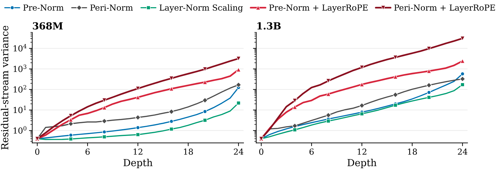
The toy is useful mostly for what it shows that the paper does not say. At 24 layers, the learned LayerRoPE schedule ends with 2.5x Pre-Norm's variance (the real 1.3B ratio in the figure above is 2,420 against 575, about 4.2x, because real block weights also grow), and its last layer's relative update is 0.297 against Pre-Norm's 0.208. A constant-factor lift, then, and no cure. Work out the sum and you see why: if the per-layer write grows as , the stream's variance grows as , and the relative update still decays like , only from a start times higher. A power-law schedule can delay the curse of depth but cannot remove it. Drag the depth slider to 512 and the extrapolated learned schedule gives a last-layer relative update of 0.065 against Pre-Norm's 0.044.
In the toy, turning the read down and the write up are the same knob, since the block is linear. The paper's reason to separate them must live in the nonlinear blocks. Attention logits scale with the square of the read gain, so a damped read keeps softmax from saturating, and SwiGLU's gate behaves differently at different input scales. A reasonable story, but the paper does not test it directly. Its evidence is the learned slopes plus the end losses.
How it was trained
The claims only mean something next to what each experiment held fixed, so I put the six setups side by side.
| Experiment | Shapes | Data, budget | Tuning | Seeds |
|---|---|---|---|---|
| Scaling ladder | 58M, 134M, 250M, 554M, 1.34B; LLaMA-style, head dim 64 | C4, 80 tokens/param, up to 107.1B tokens, sequence length 256 | LR swept per method up to 554M; 1.3B at an LR extrapolated from a power-law fit | 1 (3 at 58M and 134M) |
| Depth sweep | width 128, 48 to 512 layers, 17.8M to 111.1M params | C4, 20K steps x 512 seqs = 2.6B tokens | shared LR of 1e-3 for all methods; separate per-method sweep in Appendix D.2 | 2 up to 384 layers, 1 at 512 |
| LR basins | 58M, 368M, 1.3B, Pre and Peri, with and without LayerRoPE | C4, shorter budgets | swept over 2 to 3 orders of magnitude | 1 |
| 6.7B | LLaMA-7B shape, 32 layers, width 4096 | 11.7B tokens; schedule set for 150K steps, stopped at 89K | shared LR of 5e-4, untuned | 1 |
| Looped (Parcae) | 140M, 370M, 770M | FineWeb-Edu, 11.2B to 61.6B tokens | Parcae's recipe as-is (Muon + AdamW, clipping at 1.0) | 1 |
| ViT | ViT-T, ViT-S | ImageNet-1k, 300 epochs, DeiT recipe | none | 1 |
The ladder recipe has some unusual choices, all listed in Appendix D.1: Adam with no weight decay and no gradient clipping ("for fairness"), every document padded or truncated to 256 tokens, the norm gains kept in fp32 while everything else is bf16. At 1.3B the output logits grew until bf16 rounding destabilized late training (the final norm gain was not weight-decayed), so the authors resumed four of the five 1B runs from a pre-instability checkpoint with fp32 logits. All of that applies equally to every method, which keeps the comparison fair inside the paper. It also means the comparison is between methods on a recipe nobody would use for a real pretraining run.
Checking the 3.4x
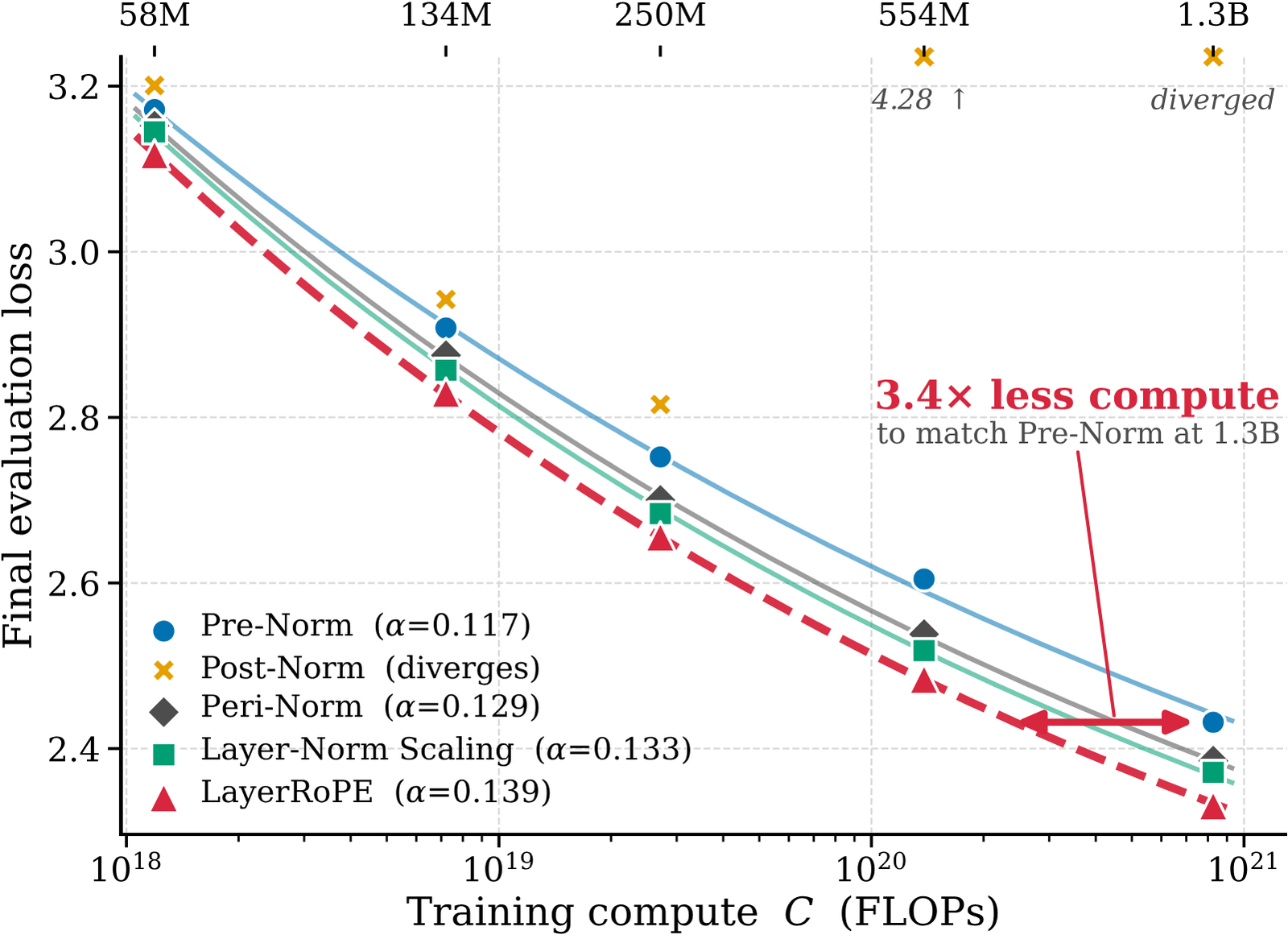
Appendix D.1.3 defines the number exactly. Fit to the 20 (method, scale) points with a shared , then divide Pre-Norm's 1B compute ( FLOPs) by the compute at which LayerRoPE's fitted curve reaches Pre-Norm's measured 1B loss. The paper notes the crossing falls between LayerRoPE's own 554M and 1.3B points, so it is an interpolation.
I redid it. I read every marker off the figure by pixel colour, calibrated against the gridlines, fixed and each method's exponent to the values printed in the legend, and refit . Pre-Norm's 1.3B point reads 2.431 and LayerRoPE's 2.324, and LayerRoPE's curve reaches 2.431 at FLOPs. That is a ratio of 3.44. The headline reproduces.
The same arithmetic against the other baselines is what the post leaves out:
- Layer-Norm Scaling reaches Pre-Norm's 1.3B loss with about 2.2x less compute, and Peri-Norm with about 1.7x less. Most of the 3.4x is something the existing fixes already buy.
- Against the strongest baseline, LNS, LayerRoPE reaches LNS's 1.3B loss (2.371 on my reading) with about 1.6x less compute. Against Peri-Norm it is about 2.1x.
- In loss terms, LayerRoPE's lead over Pre-Norm is 0.043 nats at 58M and 0.085 at 134M (three-seed means, Table 7), and about 0.127 at 554M and 0.107 at 1.3B on my reading of the plot. Its lead over LNS grows only from 0.018 nats at 58M to about 0.046 at 1.3B. Seed-to-seed standard deviation is at most 0.016 nats, so the margins are real, but the one against LNS is modest.
I trust a 1.6x over the best fix more than a 3.4x over no fix, and it is still a good result for sixteen scalars.
Three more caveats, all in the paper's own appendix:
- The curves compare methods at a fixed 80 tokens per parameter, not along a compute-optimal frontier. The paper says so. A compute saving here means "a smaller model trained the same way matches it", not "you can train the same model for less".
- The 1.3B runs are single runs at extrapolated learning rates, not swept ones. Table 6 has LayerRoPE's 1B rate at against Pre-Norm's , a ratio of 16x, not the "4 to 8x" the text gives; the 4 to 8x holds from 58M to 554M (64/16, 32/8, 64/8, 32/4).
- The downstream table supports the loss but is noisy. At 1.3B LayerRoPE's eight-task average is 52.6 against 48.0 for Pre-Norm and 51.6 for Peri-Norm, but MMLU sits between 22.9 and 23.8 for every method at every size, below the 25% you get by guessing. The average includes one task that is pure noise.
The 6.7B run is the only point beyond 1.3B, and it is weaker evidence than it looks. Every method trains for 11.7B tokens (under 2 per parameter) at a shared, untuned learning rate, and stops at step 89K of a cosine schedule set for 150K, so no run has annealed. LayerRoPE finishes 0.168 nats below Pre-Norm and 0.087 below LNS, and matches Pre-Norm's final loss after 41K steps. That tells you it is stable at 7B and ahead early in training. It does not tell you the gap survives a full run.
Checking "stable up to 512 layers"
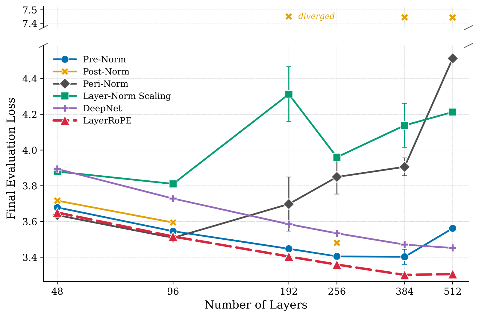
The claim survives, in a narrow regime. These models are 128 wide. At 512 layers that is an aspect ratio of 0.25, far deeper and narrower than anything anyone trains, and the whole model is 111.1M parameters, of which 8.2M is the untied 32K vocabulary. Each run sees 2.6B tokens.
LayerRoPE's loss falls from about 3.65 at 48 layers to about 3.30 at 384 and stays flat at 512. Pre-Norm trails it by 0.05 to 0.1 nats up to 384 layers and then jumps to about 3.56 at 512, on one seed. At 48 and 96 layers Peri-Norm matches or slightly beats LayerRoPE. Peri-Norm and LNS falling apart past 96 layers is the striking part of the figure; under the per-method sweep in Appendix D.2 they still degrade, so this is not a learning-rate artefact.
Two things limit what this shows. First, depth is not traded against width here: every extra layer adds about 200K parameters, so the deeper models are also bigger, and a falling loss is what you expect from any method that merely keeps training. The question DepthBench asked, whether the extra depth beats spending the same parameters on width, is not asked. Second, DeepNet runs with the prescribed for 32 layers at every depth. The authors note that this beat the depth-matched value at the shared rate, which is fair, but it is the one baseline designed for this regime and it is configured off its own recipe.
So "LayerRoPE trains stably at 512 layers" is supported. "LayerRoPE makes very deep models a good use of parameters" is not tested.
What the ablation says about the rotation
Table 4 ablates at 134M, one seed per row, and its numbers deserve more attention than the paper gives them. On the Peri-Norm backbone the baseline loss is 3.0720; magnitude only reaches 3.0351, rotation only 3.0533, and both together 3.0252. So magnitude gets about four-fifths of the full gain on its own. On the Pre-Norm backbone, replacing RoPE's frequency spectrum with one angle for every pair costs 0.006 nats (3.0317 against 3.0379), which is smaller than the seed-to-seed spread of 0.014 that Table 7 reports for Pre-Norm at the same scale. Giving each layer its own free instead of the shared one changes nothing (3.0318 against 3.0317) while adding 33.8K parameters.
I read that as: the depth-scheduled magnitude, especially the new write gain, is the method. The rotation helps a little on its own, its multi-frequency spectrum is not distinguishable from one angle at this sample size, and the shared vector is a free parameter saving rather than a source of quality. That matches what I saw in LLaMA-2's weights, where direction barely changes after layer 1. It also suggests a cheaper experiment the paper did not run: drop the rotation, keep the learned power-law read and write gains, and see how much of the 1.6x over LNS remains.
Outside language modelling
Applied untuned to Parcae, a looped model, LayerRoPE lowers validation perplexity at all three sizes: 18.66 to 18.36 at 140M, 14.22 to 14.05 at 370M, 12.49 to 12.09 at 770M. The relative gains are smaller than on the ladder, and Parcae's recipe uses Muon with gradient clipping at 1.0. That fits a suspicion I cannot test: some of the ladder's learning-rate robustness, LR sensitivity cut 3 to 10x, may be robustness to the missing clipping. The recurrent state's norm reaches about at 770M against about for plain Parcae, while its token states stay less collinear. The paper reads that as more of the loop's capacity being used. I read it as a number I would want to see survive bf16 or fp8 inference before shipping it. For the looped-model background, see the looped Transformer explainer and LoopCD, which works with Parcae too.
On ImageNet, ViT-T gains 0.9 points of top-1 (72.21 to 73.08) and ViT-S 0.6 (79.80 to 80.38), one run each with DeiT's recipe unchanged.
What is still untested
- Scale past 1.3B at a real budget. The 6.7B run is short, untuned and not annealed.
- Context length. Everything on the ladder trains on 256-token sequences. How a 4 to 100x wider stream interacts with long-context attention, sequence RoPE scaling, or attention sinks is unknown.
- A modern recipe. No weight decay, no gradient clipping and Adam rather than AdamW on the main experiments. Part of the learning-rate story may change once clipping is on.
- Inference numerics. A stream with 4 to 94x the variance of its baseline, and a looped state at around , is a quantization question the paper does not ask.
- The strongest competitors. Hyper-Connections, mHC and Attention Residuals are cited and not run, and Mix-LN is not mentioned. DepthBench suggests the redesigned streams are where depth actually pays.
- Code. None is released yet, so I could not check the implementation, the initialisation or the exact read and write placement against a source file.
What I would take from it: if you train Pre-Norm models, a learned power-law gain on each block's output, initialised at a negative slope and allowed to go positive, is about the cheapest experiment in this whole area: parameters, under 0.02% of the FLOPs. The paper's evidence that it beats Layer-Norm Scaling at 1.3B is solid. The evidence that the RoPE-style rotation is what makes it work is thin.
How I checked
I read the full arXiv HTML (v1) including all appendices and rendered the paper's figures from their source SVGs. LLaMA-2 7B's 64 RMSNorm vectors came from NousResearch/Llama-2-7b-hf through safetensors range requests; I computed per-layer RMS, the power-law fit, the angles between vectors in , and a classical MDS of the vectors and of a pure-scaling control. For the 3.4x I located Figure 1(b)'s markers by colour, calibrated against its gridlines, refit with the paper's and its printed exponents, and solved for the crossing compute; readings off a plot carry roughly ±0.003 nats of error. The parameter and FLOP counts were recomputed from Appendix A's formulas, and the learning-rate ratios read from Table 6. The two widgets use the slopes printed in Figures 20 and 21, with layer-0 values read off those plots by eye; the toy stream is labelled as one. The code above is mine, checked only for shape, norms and sign flips. No authors' code exists to compare against.