2026-09-26 · 22 min · explainer · llm · architecture · transformers · pretraining · scaling-laws · mixture-of-experts

Every Transformer carries one vector per token from layer to layer, and every layer adds its output to it. Hyper-connections replaced that single vector with several. DeepSeek's mHC made the several stable at 27B by forcing the matrix that mixes them to be doubly stochastic. Every shipped model whose config this site has read, from GLM-5.3-Flash to Magi-2, uses four streams. xHC asks why four, finds two reasons, and goes to sixteen.
The paper is from Junchi Yan's group at Shanghai Jiao Tong's School of AI with Xiaohongshu's Dots Studio. First author Xiangdong Zhang (@aHapBean) announced its NeurIPS 2026 acceptance on 25 September, with an accurate summary: "16 residual streams, reading all but updating only 4 at a time."
I read the paper, its tech report and the two papers it builds on, checked its formulas and tables in numpy, and built a toy of the mixing. Numbers are labelled Reported (the paper says it), Measured (I ran it) or Reasoned (I derived it).
| What it is | 16 residual streams, 4 mixed and written per sublayer, with a causal-conv-enriched write |
| Models | DeepSeekMoE-style, 144 experts, top-8: 18B total / 1.7B active and 28B / 2.7B for the main results; 2.5B for the N-sweep, 10B for ablations |
| Baselines | a plain residual, and mHC at N = 4. HC itself is not run |
| Benchmarks | 12 (MMLU, MMLU-Pro, MMLU-Redux, BBH, CommonsenseQA, ARC-C, GSM8K, HumanEval, LCBench, CMMLU, CEval, C3) via OpenCompass |
| Headline | average 48.8 against mHC's 44.8 at 18B, 53.6 against 50.5 at 28B |
| Training tokens | not reported, for any model |
| Code | none yet: aHapBean/xHC holds a README, seven images and the tech report PDF |
One stream: x + F(x)
A residual block computes . Unroll it and the top of the network is the input plus a sum of every layer's contribution:
The identity in that Jacobian is the whole trick. However badly the layers behave, the gradient reaching layer has a path that multiplies by exactly 1, so depth does not by itself make signals explode or vanish. That is why a deep stack trains at all.
The cost is width. One -dimensional vector carries everything, and every layer writes into the same numbers.
Hyper-connections: N streams, three small maps
Hyper-Connections (Zhu et al., ByteDance) copy the embedding into streams, so the state is a matrix . The layer still sees one -vector, so its cost does not change. Three small learned maps sit around it:
reads the layer's input as a weighted sum of streams. writes the output back with one weight per stream. mixes the streams with each other. HC calls these width and depth connections; I use mHC's names. In the dynamic variant each map is predicted from the current state. With and all three maps fixed at 1, this is the plain residual again.
Reported by HC, on OLMo-1B trained for 500B tokens (its no-tanh variant): is worse than the baseline, and are better, and reaches a validation loss of 2.777 against 2.779 at , with 63.8 average downstream accuracy against 64.4. The saturation xHC sets out to fix was visible in the first paper.
The problem is that is unconstrained, and a signal crossing many layers is multiplied by . Nothing stops that product growing or shrinking geometrically: the identity path is gone. Reported by the mHC paper: in a 27B model, HC's loss surges around step 12k, in step with its gradient norm, and the gain of the composite mapping, its largest absolute row or column sum, reaches nearly 3000.
mHC: keep the mixing doubly stochastic
mHC (Xie et al., DeepSeek) constrains to the Birkhoff polytope: non-negative matrices whose rows and columns each sum to 1. It gets there with Sinkhorn-Knopp. Exponentiate the predicted logits, then alternately rescale columns and rows, 20 times:
Three properties follow. Each output stream is a convex combination of input streams, so nothing is amplified and the mean across streams is conserved. The spectral norm is at most 1. And doubly stochastic matrices are closed under multiplication, so the product across any depth is doubly stochastic too: whatever the network learns, the composite mixing cannot amplify. mHC also bounds the other two maps, a sigmoid on and on .
Reported by mHC: at 20 iterations the constraint is approximate, and the composite backward gain peaks around 1.6 against HC's nearly 3000. Training overhead at is 6.7%. This is the operator GLM-5.3-Flash ships as hc_mult: 4, hc_sinkhorn_iters: 20, the one Magi-2 runs in Triton and the one Qwen's Gated Residual deleted; Chimera and Hy4 fix it to the identity. The GOAT article steps through Sinkhorn one half-step at a time.
One detail matters later. mHC's Eq. 9 normalizes rows last, so every row sums to exactly 1 and the approximation error lands on the columns. That is why mHC measures the backward gain drifting, not the forward one.
| rule | streams | forward | backward | self-share |
|---|---|---|---|---|
| plain residual | 1 | 1.000 | 1.000 | 1 |
| HC (unconstrained) | 16 | 5.4e4 | 4.7e4 | n/a |
| mHC (Sinkhorn) | 16 | 1.000 | 1.000 | 0.063 |
| xHC (k of N) | 16 (4 active) | 1.000 | 1.008 | 0.518 |
Self-share is the average diagonal of the product: how much of each stream's own sublayer-0 content it still holds at the top. It is only meaningful for a doubly stochastic product, where 1 means the streams never mixed and 1/N means every stream has become the average of all of them.
The widget keeps only the mixing. Each sublayer draws one random matrix . HC uses it as is, mHC uses Sinkhorn of , and xHC applies that Sinkhorn to a routed block and leaves the other streams alone. The chart tracks the product's gain the way mHC measures it: largest absolute row sum (forward) and column sum (backward).
Measured, on the widget's default draw at 64 sublayers and drift 0.15: HC's forward gain reaches 4.05 with four streams and about 54,000 with sixteen. mHC and xHC sit at exactly 1.000 forward. Backward they come out at 1.012 and 1.014 with four streams and 20 iterations. Cut Sinkhorn to one iteration and sixteen streams give 1.143 and 1.148. With four streams, bias -0.05 and drift 0.1, HC vanishes to 0.157 and the Sinkhorn rules do not move. That is the argument for mHC in one picture, on random matrices, not a trained model.
The widget also shows something the stability argument leaves out. A product of doubly stochastic matrices with positive entries converges to the matrix whose every entry is : every stream becomes the average of all of them. Measured in the toy: after 64 sublayers, dense mHC's self-share, the average diagonal of the product, is 0.252 with four streams and 0.063 with sixteen, which is in both cases. Reasoned: under this constraint, mixing only ever pulls streams together, and the only thing that keeps them apart is what each layer writes.
Why mHC stops at four
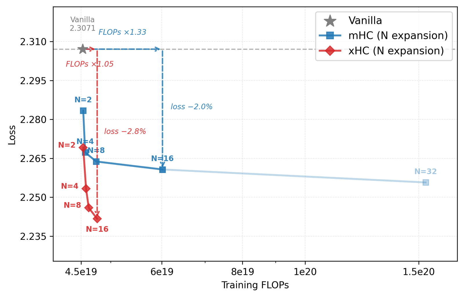
Reported, on the 2.5B model: taking mHC from 4 streams to 16 lowers loss by 0.006 and raises training FLOPs by 32%. xHC over the same range lowers it by 0.012 for 4%. The paper names two bottlenecks.
Information. mHC's write to stream is : a scalar times the one output vector. Across all streams the update is an outer product , rank one. Sixteen streams can weight each layer's single vector sixteen ways, but they cannot receive sixteen different things. The paper's word for the result is redundant, and the averaging above is one reason why (Reasoned).
Cost. is predicted from the flattened -dimensional state by . That is weights per sublayer. At it is , at it is . The layer itself does not get more expensive; the generator of its mixing matrix does.
What xHC changes
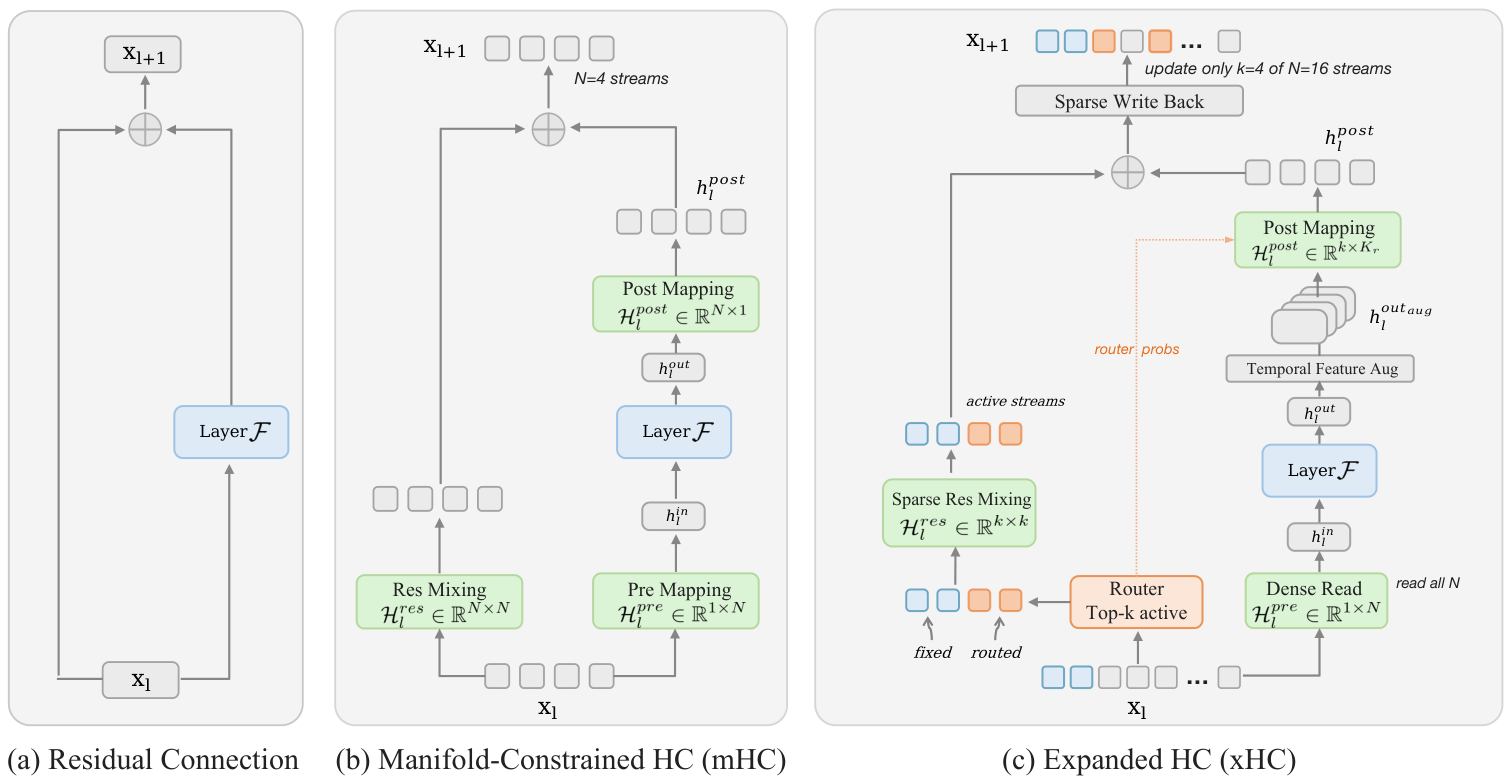
xHC makes three changes to one sublayer.
Dense read. still reads every stream, so every layer can see all sixteen.
Sparse mix and write. A router scores all 16 streams per token, . Streams 0 and 1 are always active; the top 2 of the other 14 by score join them, in all. The mixing matrix is generated from those four streams only, , and the four are updated:
The other 12 streams pass through untouched. Routing is per token, like MoE: two tokens in the same sequence can write different streams. The router weights (1 for the fixed streams, the sigmoid score for the routed ones) scale only the write. The paper is explicit that mixing stays ungated.
A richer write. After MLP sublayers only, the output is convolved causally along the sequence with three depthwise kernels of width 4, 8 and 12. The three results are Gram-Schmidt-orthogonalized against the output and each other, giving components . That costs parameters per MLP sublayer, and the tech report adds that the kernels start at zero, so training begins with mHC's single write.
Here is the whole sublayer as runnable numpy, with the learnable scale and biases left out. On random weights it touches exactly four streams per token, and with the write zeroed the sum over streams is conserved to 3.6e-15 (Measured).
import numpy as np

sig = lambda z: 1 / (1 + np.exp(-z))
rms = lambda x: x / np.sqrt((x * x).mean(-1, keepdims=True) + 1e-6)

def sinkhorn(logits, iters=20):              # mHC Eq. 9: columns, then rows
    M = np.exp(logits - logits.max((-2, -1), keepdims=True))
    for _ in range(iters):
        M = M / M.sum(-2, keepdims=True)
        M = M / M.sum(-1, keepdims=True)
    return M

def xhc_sublayer(X, F, W, k=4, m=2, convs=()):
    """X: (S, N, C) state for S tokens. F: attention or MLP, (S, C) -> (S, C).
    convs: causal depthwise kernels, each (kappa, C); empty for attention."""
    S, N, C = X.shape
    flat = X.reshape(S, N * C)
    # route, per token: m fixed streams + top (k - m) of the rest
    ln = (flat - flat.mean(-1, keepdims=True)) / (flat.std(-1, keepdims=True) + 1e-6)
    s = sig(ln @ W["router"])
    top = np.argsort(-s[:, m:], -1)[:, : k - m] + m
    idx = np.concatenate([np.tile(np.arange(m), (S, 1)), top], -1)
    p = np.concatenate([np.ones((S, m)), np.take_along_axis(s, top, -1)], -1)
    # dense read over all N streams
    out = F(np.einsum("sn,snc->sc", sig(rms(flat) @ W["pre"]), X))
    # temporal augmentation: causal convs, then Gram-Schmidt
    comps = [out]
    for w in convs:
        pad = np.concatenate([np.zeros((len(w) - 1, C)), out])
        g = sum(w[i] * pad[len(w) - 1 - i : len(w) - 1 - i + S] for i in range(len(w)))
        for v in comps:
            g = g - (g * v).sum(-1, keepdims=True) / ((v * v).sum(-1, keepdims=True) + 1e-6) * v
        comps.append(g)
    aug = np.stack(comps, 1)                                   # (S, K_r, C)
    # mixing and write maps from the k active streams only
    Xa = np.take_along_axis(X, idx[..., None], 1)              # (S, k, C)
    xa = rms(Xa.reshape(S, k * C))
    H_res = sinkhorn((xa @ W["res"]).reshape(S, k, k))
    H_post = 2 * sig((xa @ W["post"][len(comps)]).reshape(S, k, len(comps)))
    Xa = H_res @ Xa + p[..., None] * (H_post @ aug)            # mix, then gated write
    X = X.copy()
    np.put_along_axis(X, idx[..., None], Xa, 1)                # 12 streams untouched
    return X
What "more expressive" and "greater capacity" mean
Capacity is the persistent state: numbers per token instead of mHC's , and a stream that routing skips keeps its contents for later layers to read.
Expressiveness is the rank of the write. mHC adds a rank-one matrix to the state per sublayer. xHC's MLP sublayers add , which has rank up to 4, and three of those four directions carry information from the previous 3, 7 and 11 tokens. Attention sublayers still write rank one. The mixing per sublayer is not more expressive: a doubly stochastic block has the same freedom as mHC's at , applied to a routed subset.
Which constraint survives
All of it, and this is the part I like best. Reasoned: one sublayer's effective map is the Sinkhorn block on the active streams and the identity on the other 12, conjugated by a permutation. A block-diagonal of doubly stochastic blocks is doubly stochastic, and permuting rows and columns together preserves both sums. So every sublayer's full mixing matrix is doubly stochastic, and so is the product over depth: mHC's guarantee carries over to sixteen streams without a Sinkhorn. The toy agrees: xHC's forward gain stays at 1.000 at every setting. It also keeps more of each stream apart, with a self-share of 0.518 at sixteen streams against dense mHC's 0.063 on the same draw (Measured, toy only).
What xHC relaxes is density: in any one sublayer, 12 streams take no part in mixing. It adds one patch. Reported in Appendix A: "rare extreme activations can hinder the convergence of Sinkhorn normalization, leaving some row sums greater than one," so rows are rescaled by after Sinkhorn. Reasoned: with mHC's column-then-row order, rows come out exactly 1 and this clamp could never fire. Either xHC's kernel normalizes in the other order, or the failure is numerical. The paper does not say which.
What it costs
At N = 16, k = 4, xHC carries 1,256 C parameters per layer: 7.3x fewer than dense mHC at the same N and 6.5x more than mHC at N = 4. 82% of it is the router and read map, which still grow as N².
Parameters, from Appendix C, per layer in units of : mHC at is , mHC at is , xHC at is . I reproduce all three. xHC has 7.3x fewer than dense mHC at the same and 6.5x more than the mHC anyone ships. Reasoned: of xHC's , or 82%, is the router and the read map, both of which still read the full state and grow as . The cubic term is solved; the quadratic one is next.
FLOPs. Reported: xHC adds 4.1% training FLOPs at 18B and 3.0% at 28B, against 0.7% and 0.5% for mHC at . Reasoned, applying Appendix C's own recipe to Table 6's configurations: it reproduces the 28B column (my 0.46%, 22.2% and 3.0% for mHC-4, mHC-16 and xHC, against their 0.5%, 22.3% and 3.0%) and the 2.5B sweep (+30% for mHC from 4 to 16 streams against their 32%, +3.7% for xHC against their 4%). It cannot reproduce the 18B column, and nothing can: mHC-16's and xHC's overheads are both over the same backbone, so their ratio must be , and the table has . The recipe gives 3.3% for xHC and 24% for mHC-16 at 18B. Both errors run against xHC, so the slip is not self-serving, and the real overhead is small either way.
Memory traffic is what the step time pays for. Reported (Table 4), per token per sublayer: a plain residual moves , mHC at moves , xHC , dense mHC at would move . I re-derived all four from the table's rows. xHC reads the full state twice per sublayer, to generate maps and for the dense read. xHC-Flash shares routing and both reads across an attention-plus-MLP block, drops the attention-side mixing, and corrects the MLP's input exactly with one scalar, : . xHC-Flash-4sub shares across two blocks: . At 10B the three reach validation losses of 1.983, 1.983 and 1.984.
Residual memory. Reasoned: the state is per token. In bf16 at the 18B model's that is 67,584 bytes per token for sixteen streams, against 16,896 for four and 4,224 for one: four times mHC's, at every layer boundary a framework keeps for backward. The paper reports traffic, not peak memory.
Wall clock. Reported, on the 18B model with pipeline overlap off: the authors' fused mHC adds about 15% over vanilla (DeepSeek reported 6.7%; the paper says the setups differ), and xHC-Flash-4sub about 11% on top of mHC. Prefill at 2K tokens costs 11.4% over vanilla for mHC and 12.9% for xHC-Flash-4sub. Full xHC, the model behind every downstream score, is never timed; xHC-Flash-4sub, the one that is, has one validation loss at 10B and no benchmarks.
Reasoned, roughly: xHC-Flash-4sub's step costs 1.26x to 1.28x vanilla's (15% and 11% may add or compound) for about 1.04x the FLOPs. Charge the scaling-law multipliers below at that rate and 1.50x over vanilla becomes about 1.2x, and 1.19x over mHC about 1.1x: still a win, smaller than the FLOPs axis shows, assuming full xHC's fits carry over to Flash-4sub.
What the results say
Setup, reported. AdamW, 8,192 context, a mix of English, Chinese, code, maths and reasoning data, matched recipes per scale. Table 6 lists "Training Tokens" as a dash for every model, and the 18B global batch too; its loss curve runs to about 46,000 iterations. Reasoned: the 2.5B sweep's vanilla point sits at 4.5e19 FLOPs in Figure 1, and Appendix C's recipe gives about 2.8 GFLOPs per token for that model, so roughly 16B tokens. The same recipe puts mHC at 32 streams at 3.3x vanilla's FLOPs, where Figure 1 draws it. For 18B and 28B I cannot estimate.
Downstream, reported (Table 1). Single runs, no error bars.
| Vanilla | mHC (N = 4) | xHC (16, 4) | xHC − mHC | |
|---|---|---|---|---|
| 18B average | 40.6 | 44.8 | 48.8 | +4.0, wins 12 of 12 |
| 28B average | 47.8 | 50.5 | 53.6 | +3.1, wins 11 of 12 |
| 18B final training loss | 1.799 | 1.776 | 1.758 | −0.018 |
At 28B the one loss is BBH, 43.4 against 43.6. The largest gains at 18B are HumanEval (+6.1), ARC-Challenge (+5.9) and BBH (+5.8). At 28B they are CommonsenseQA (+5.7), HumanEval (+4.3) and C3 (+3.8). mHC itself scores below vanilla on HumanEval at both scales (23.2 against 25.6, and 26.8 against 27.4) and on LCBench at 28B.
Does the gain hold at the largest scale? It holds, and it shrinks. Over mHC it goes from 4.0 points to 3.1, and over vanilla from 8.2 to 5.8 (Reasoned from the table). mHC's own lead over vanilla shrinks too, from 4.2 to 2.7. Two points on a curve cannot say whether that trend continues.
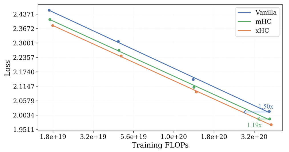
Scaling law, reported. Four models per method, 1.7e19 to 4.0e20 FLOPs, the largest 1.10B active and 9.46B total. Fits of give exponents of 0.0936 (vanilla), 0.0920 (mHC) and 0.0919 (xHC). The largest measured vanilla and mHC losses, read against the fitted xHC line, give the headline 1.50x and 1.19x.
Reasoned, from Table 9's own parameters: the three exponents agree within 0.0017, and mHC's and xHC's within 0.0001, so xHC shifts the curve down and does not make it steeper. It is a constant-factor saving. Fit against fit at 4.0e20 FLOPs the multipliers are 1.41x and 1.11x, a little under the headline, because the largest baseline points sit slightly above their own lines. Across the measured range the vanilla multiplier narrows from 1.49x to 1.41x; the mHC one holds near 1.11x. Four points per fit cannot resolve a 0.0017 exponent gap, so I would not extrapolate.
Muon, reported. On the 18B model with Muon on the backbone, xHC lifts the average from 43.1 to 49.9 (without Gram-Schmidt, which the authors found unnecessary under Muon). There is no Muon-plus-mHC run, so this shows xHC works with Muon, not its margin over mHC there.
Where the loss actually comes from
Reported, Table 2, at 10B on the Pile test set: vanilla 2.029, mHC at 2.004, mHC at 1.998, mHC-16 with temporal augmentation 1.984, full xHC 1.983. Sparse routing costs nothing in loss and cuts the FLOPs overhead from 20.1% to 3.3%. Keeping two fixed streams and the dense read matters: drop both and loss rises to 1.997. gives 1.991, gives 1.982, a softmax router 1.988.
Reasoned: of the 0.021 that separates mHC at four streams from xHC, 0.006 comes from widening to sixteen and 0.014, two-thirds, from the causal convolutions.
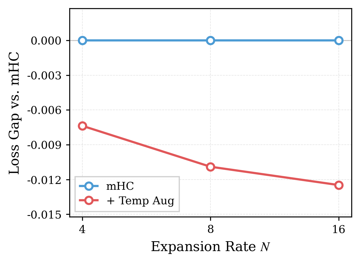
The paper reads Figure 5 as the convolution's gain growing with , which supports the information-bottleneck diagnosis. It does, from about 0.007 at four streams to about 0.0125 at sixteen (read off the plot). The other reading is that more than half of it is available at four streams, with no expansion at all. The 18B and 28B comparisons never include mHC-4 with the convolution, or a plain residual with one. So the 4.0 points bundle two ideas: more streams, and a short causal conv on the MLP output, a token-mixing change in its own right. The ablation says both are real at 10B, not how the downstream points split.
Stability, read closely
xHC inherits mHC's structural bound, but not mHC's evidence: no gradient-norm curves and no composite-gain plots. The 18B loss curves in Figure 2(a) are smooth, but the plot starts around iteration 5,000. The stability story is told instead by the fixes it needed:
- Row-sum clamping after Sinkhorn (Appendix A, above).
- Gram-Schmidt is load-bearing at scale. At 10B, removing it barely moves the loss (1.984 against 1.983). At 18B, "the cosine similarity between convolutional branches and the main branch can exceed 0.7, and removing Gram–Schmidt orthogonalization leads to training instability."
- No convolution after attention. Section 3.3.1 says it "empirically destabilizes training." Appendix D's 10B ablation reports "a similar validation loss," 1.985 against 1.983, slightly worse. Both can be true at different scales, but the paper shows only the mild one.
- Two fixed streams, described as providing "guaranteed write targets" for stability.
None of this is alarming, and the paper is candid about each fix. It means reproducing xHC takes those four fixes, not just the equations.
What I could not check
No code. The repository at commit 7890266 (21 July) holds a README, figures and paper/xHC_tech_report.pdf; the README links xHC_technical_report.pdf, which does not exist. The author's post promises code "within two months." Until then the fused kernels, the Sinkhorn order, the clamp and the Gram-Schmidt epsilon are unverified. That epsilon matters: with zero-initialized kernels, Eq. 5 divides zero by zero at the first step.
Token budgets, seeds and the throughput of full xHC are not reported. The 18B FLOPs column does not add up, though both errors run against xHC, not for it.
What holds: the mechanism is clean. It keeps mHC's doubly-stochastic guarantee over all sixteen streams while paying for a Sinkhorn, and it attacks a real limit of mHC, a rank-one write per layer, not only its cost. Against mHC at matched recipes it is ahead at both scales and across the fitted compute range. I read that lead as a constant-factor gain, partly from a causal convolution, that costs more wall clock than FLOPs. I would want the mHC-plus-conv baseline before crediting all of it to sixteen streams.