2026-10-06 · 19 min · looped-transformers · inference · reasoning
Why read this
Notabletop 60%LoopCD as contrastive decoding with the first loop as the amateur, why disagreement beats accuracy for the reference, and why the 73% and 48% are separate runs.
- Original analysis
- Runs on a consumer GPU
- A lasting reference
Inference & servingResearch paper
How this was scored
- Is it new?
- 2 of 3: A real new idea, method or capability
- Can I trust it?
- 2 of 3: Measures key facts from files, code or configs
- Can I run it?
- 2 of 3: Open code or weights with real limits
- Will I understand it?
- 2 of 3: Mechanism from first principles with figures
- Can I act on it?
- 2 of 3: A concrete recipe, numbers or comparison
- Will it last?
- 2 of 3: A reference for a year or more
- Does it affect many?
- 1 of 3: A specialist community
- Only here?
- 2 of 3: A teardown or measurement few others did
Score 66 of 100, ranked 149 of 445 rated articles. Each question is answered 0–3 by hand, and a 3 is rare. How articles are scored
A looped transformer computes the same next token several times over. Each pass through its shared block produces a hidden state that the output head could decode, and ordinary decoding reads only the last one. The earlier states are computed, paid for, and dropped.
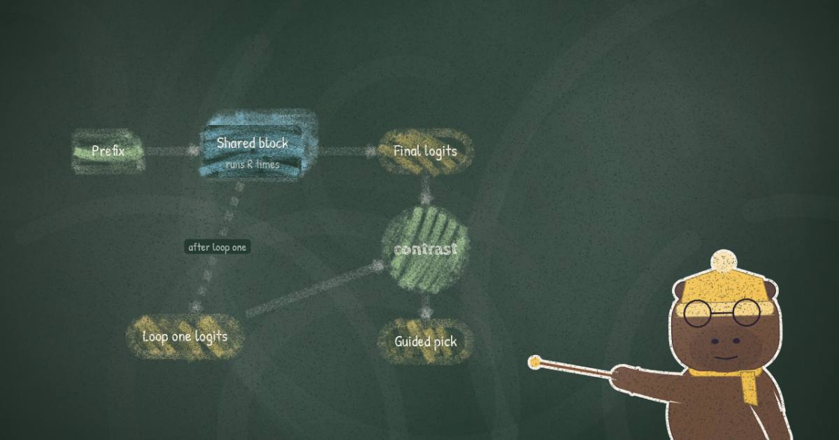
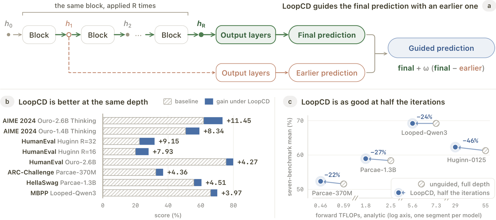
Decoding Looped Transformers Better for (Almost) Free (Liu, Zheng, Chen, Dilip, Bai, Jiao, Wang, Zhang; Apple, 1 October 2026) picks one of them back up. Its method, LoopCD, decodes the state after the first loop as well, treats it as a weak model's opinion, and pushes the final prediction further away from it. That is contrastive decoding, with the amateur model already inside the expert.
The paper reached me through a Chinese-language post on X that summarised it as: zero training cost, compute cut by 47%, math pass@1 up from 61% to 73%. The first is true. The other two are real numbers from two different experiments, and the post reads as if one run delivered both. Below: what a loop is, what contrastive decoding is, why a loop makes the amateur free, what the paper measured, and where the two headline numbers actually come from.
Every number here is labelled. Reported is the paper's figure, which I did not re-run (there is no code release I could find). Reasoned is my own arithmetic on reported numbers. Measured is something I computed from a file; in this article that is only the toy widget's arithmetic.
A looped transformer, in one equation
A standard transformer buys depth with parameters: 48 layers means 48 sets of weights. A looped transformer stores a block once and runs it times, feeding each pass's output back in. The site's architecture explainer covers the design space; the short version is two layouts.
- Loop the whole stack. Ouro runs its full decoder 4 times: Ouro-1.4B is 24 layers looped to 96 layer applications, Ouro-2.6B is 48 layers looped to 192 (reported, Table A1). Only the final norm and vocabulary head sit after the loop.
- Prelude, loop, coda. Huginn-0125 embeds the input through 2 prelude layers, iterates a 4-layer core 32 times by default, and decodes through a 2-layer coda: 132 layer applications at (reported). Parcae and Looped-Qwen3 use the same sandwich. Looped-Qwen3 is a retrofit (Training-Free Looped Transformers): a frozen Qwen3-4B with a 4-layer middle window repeated as damped substeps, 15 layers before it and 17 after (reported).
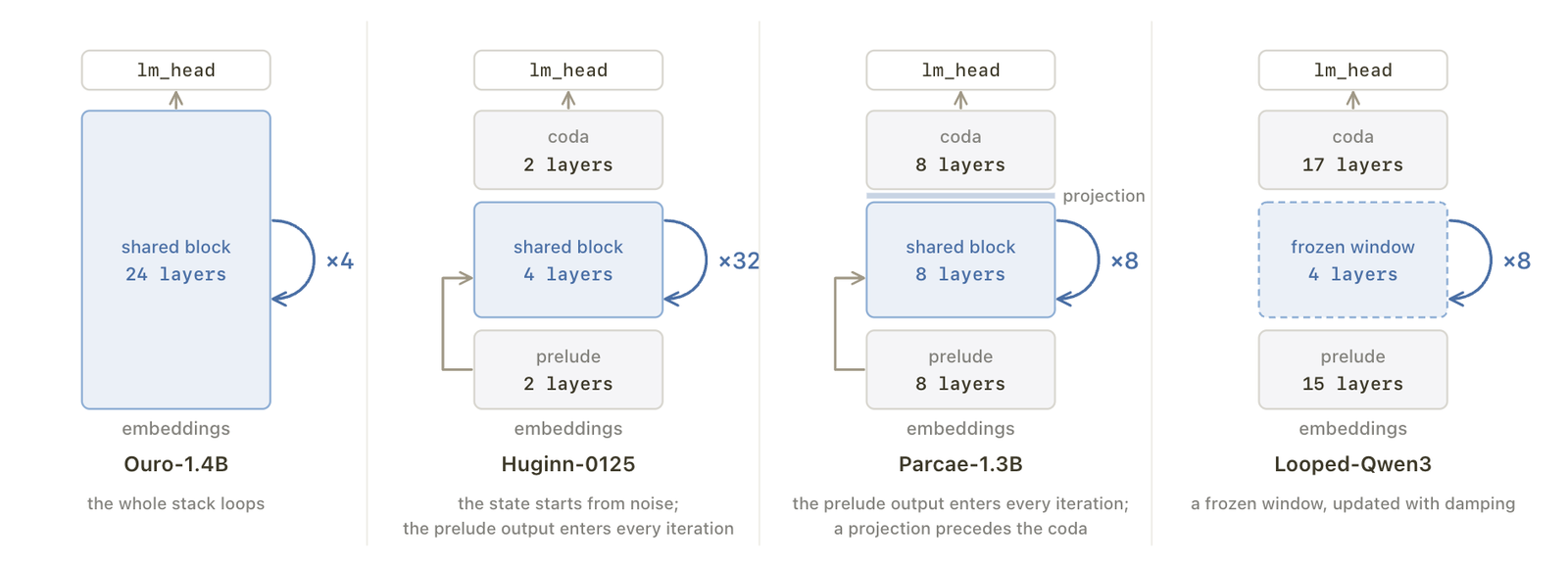
The paper writes all four the same way. Let be the state entering the loop and the shared update:
is the vector of next-token logits, and decoding samples from . The point that makes this paper work: lives in the same space as , because the same block wrote both. So is a legitimate next-token distribution too. It is just a worse one.
How much worse is reported in Figure 5 and Table A11. On the seven-benchmark multiple-choice mean, the prediction after the first loop trails the final one by 4.0 to 23.7 points across six models (reported). On ARC-Challenge, Huginn's first step scores 22.78% against 37.54% for its final prediction; Ouro-1.4B's first pass scores 38.65% against 60.41% (reported).
Contrastive decoding, from the original
Contrastive decoding (Li et al., 2022) starts from an observation about failure modes. A large language model and a small one make many of the same mistakes: repetition, generic continuations, the most frequent token. Where the large model's preference differs from the small one's is where its extra capacity shows. So score each candidate token by the difference:
A pure difference has an obvious bug: a token both models consider nearly impossible can win, because is a big ratio. Li et al. guard against that with a plausibility constraint: only tokens with are eligible, with .
O'Brien and Lewis (2023) rewrote it with a strength knob so it degrades gracefully to ordinary decoding, using expert logits and amateur logits :
is the expert alone; they used and kept , and reported gains on GSM8K and HellaSwag with LLaMA-65B as the expert. The practical problem with all of this is the amateur. You need a second model that shares the tokenizer, makes the same kind of mistakes, and is cheap enough to run alongside the expert at every step. DoLa dodged it by using an early layer of the same model as the amateur, which needs that early layer to be decodable.
LoopCD: the amateur was already computed
A looped transformer supplies an aligned amateur for nothing. is the same model, on the same prefix, after one loop's worth of compute instead of . LoopCD-Logits decodes both and extrapolates:
Rearranged, : exactly O'Brien and Lewis's form with , the final loop as expert and the first loop as amateur. The paper's Appendix A.3 states the probability form, . Read it as: keep the final distribution, then multiply each token by how much the loops raised it, to the power .
There is no plausibility mask in the paper's equations (Appendix A.3 says its identity describes the logits "before any temperature or truncation used by an evaluation protocol"). Its guard is a different one: an adaptive strength that sets per token from how close the final prediction's top two candidates are,
so a confident token gets almost no push and a coin-flip gets the full .
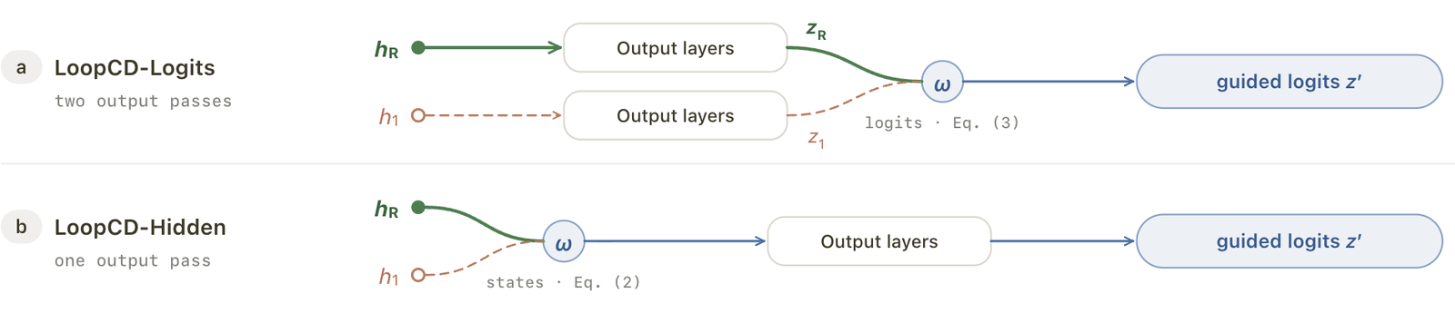
The second form, LoopCD-Hidden, applies the same extrapolation to the states before the coda, , and decodes once. It costs no extra output pass. It is not the same function: the coda is nonlinear, so the probability identity above does not hold for it, and the adaptive rule needs , which LoopCD-Hidden never computes. The paper runs LoopCD-Hidden at fixed strength only.
The widget below runs LoopCD-Logits on six invented tokens. The final loop slightly prefers "12" (logit 2.3) over "15" (1.9); the first loop preferred "12" by much more (2.5 against 0.8). Between loop one and loop , "15" gained 1.1 logits and "12" lost 0.2, so the contrast favours "15", and once passes about 0.31 the argmax flips (0.4 logit gap, divided by 1.3 of relative motion). A junk token, "banana", shows why Li et al. needed : the first loop gave it a logit of −4.2 and the final loop −0.6, so its contrast of +3.6 is the largest in the vocabulary. Push past 1.0 and it wins. An of 0.06 or more masks it; the adaptive rule only delays it. These logits are illustrative; the arithmetic is the paper's Eq. 3 and Eq. 4.
| token | z₁ | z_R | z_R − z₁ | probability: first loop · final loop · guided |
|---|---|---|---|---|
| 12 | 2.5 | 2.3 | -0.2 | 59.8% 47.5% 33.4% |
| 15 ◂ | 0.8 | 1.9 | +1.1 | 10.9% 31.8% 42.8% |
| 20 | 0.7 | 0.6 | -0.1 | 9.9% 8.7% 6.4% |
| x | 0.9 | 0.2 | -0.7 | 12.1% 5.8% 3.2% |
| so | 0.4 | -0.3 | -0.7 | 7.3% 3.5% 1.9% |
| banana | -4.2 | -0.6 | +3.6 | 0.1% 2.6% 12.3% |
The guided pick flips from "12" to "15". The final loop preferred "12" by 0.4 logits, but between the first loop and the last, "15" gained 1.1 while "12" lost 0.2, so continuing that motion closes a 0.4 gap at ω ≈ 0.31.
Bars, top to bottom: the first loop's softmax(z₁), the final loop's softmax(z_R), and the guided softmax(z′) with z′ = z_R + ω(z_R − z₁). Toy numbers chosen to show the mechanism; none of them come from the paper.
What the paper's own example looks like
The paper traces one ARC-Challenge question through Ouro-1.4B (Table A13, reported): which natural disaster leaves a narrow path of destruction through a forest. Per-character log-likelihoods:
| option | after the first pass | final | guided, |
|---|---|---|---|
| a flood | −1.500 | −0.770 | −0.934 |
| a tornado (correct) | −1.113 | −0.209 | −0.170 |
| a hurricane | −0.969 | −0.258 | −0.247 |
| an earthquake | −0.525 | −0.201 | −0.199 |
The final pass picks "earthquake" by under 0.01. Across the passes, "tornado" rose by 0.90 and "earthquake" by 0.32; continuing that motion puts "tornado" first. The guided column is not applied to these four numbers, because guidance acts on every token of every option's continuation and each token is renormalised over the whole vocabulary; the option score is the sum afterwards. Same idea, one level down.
Why the first loop, and not a later one
The intuitive choice for an amateur might be the loop just before the end: nearly as good, so a gentler, safer contrast. The paper's sweep says the opposite, and the reason is useful. What the reference supplies is a direction, and a late loop that has already converged on the final answer has no direction left to give.
Table A11 (reported) lists, for each reference loop , its own accuracy, how often it picks a different answer from the final prediction, and the LoopCD-Logits gain at . On ARC-Challenge, Huginn's first step disagrees with the final prediction on 51.3% of questions and gives +3.07 points; its sixteenth disagrees on 7.3% and gives +0.17. Parcae-1.3B's sixth step is more accurate alone than the final prediction (41.04% against 40.36%) and gives +1.02, against +3.50 from its first. Huginn's second step is as weak as its first (22.10% against 22.78%) yet gives about half the gain, because it already agrees more with the end. Gain tracks disagreement, not competence.
unguided final prediction: 37.54% · LoopCD-Logits at ω = 0.5
| ref k | alone | disagrees with final | gain (points) |
|---|---|---|---|
| h1 | 22.78% | 51.3% | +3.07 |
| h2 | 22.10% | 46.8% | +1.79 |
| h4 | 30.12% | 35.8% | +0.94 |
| h6 | 32.25% | 29.5% | +1.11 |
| h8 | 33.45% | 20.0% | +0.60 |
| h16 | 37.20% | 7.3% | +0.17 |
| h24 | 38.05% | 2.7% | +0.17 |
The gain follows the disagreement column, not the accuracy column: a reference that is nearly as accurate as the final prediction, but agrees with it, has no direction left to give. Reported numbers, ARC-Challenge and HellaSwag only.
One exception, and it is instructive. Huginn initialises its recurrent state with Gaussian noise. Its first step mostly removes that noise: the paper reports the state's norm stays at 76.4 within a spread of 0.05 across all 32 steps, while the path it walks is 6.0 times longer than its net displacement (reported, Appendix E.1). The coda projects the noise away, so is a fine logit reference. But LoopCD-Hidden contrasts the raw states and amplifies that noise: early states cost 0.58 points on Huginn, and the hidden-state gain peaks at the sixth step with +0.83 (reported). So the paper's Huginn LoopCD-Hidden runs use or . Parcae and Looped-Qwen3 start from deterministic states and use in both forms.
Layers inside a pass are not a substitute. A DoLa-style reference taken from a mid-pass layer of Ouro dropped ARC-Challenge accuracy by up to 20.6 points on Ouro-1.4B and 24.9 on Ouro-2.6B (reported, Appendix E.3); within a pass, the decoded distribution swings to 0.57 to 0.84 bits of Jensen-Shannon divergence from the final one. In the paper's words, looped architectures "do not form trained exit points inside a pass"; the end of a completed loop is the natural one.
What the contrast actually does: re-rank close calls
The paper splits the logit contrast into a part parallel to and a part orthogonal to it. The parallel part scales every logit by the same factor: a temperature change that sharpens the distribution without reordering it. The orthogonal part reorders. On HellaSwag, the orthogonal part alone gives +1.72 points on Ouro-1.4B at against +0.76 for the full update (reported). Sharpening is not where the gain lives.
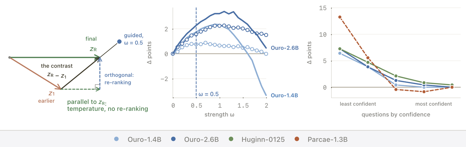
A re-ranking can only flip a decision when its push exceeds the gap between the top two options. So the gain concentrates where the model is undecided. Splitting ARC-Challenge into fifths by that gap, guidance at adds +6.4 to +13.3 points on the least confident fifth across four models and at most +0.4 on the most confident (reported). Only 5.8% to 14.9% of ARC-Challenge answers change at all (reported). This is a tie-breaker that continues the direction the loops were already moving in. It adds no knowledge; if the loops were heading the wrong way, it follows them.
The results, at full depth
Mathematical reasoning (Ouro-Thinking, sixteen samples per problem, Table 1a, reported). Ouro-2.6B-Thinking with adaptive LoopCD-Logits ():
| benchmark | baseline pass@1 | LoopCD pass@1 | change |
|---|---|---|---|
| AIME 2024 | 61.88 | 73.33 | +11.45 |
| AIME 2025 | 49.58 | 56.88 | +7.30 |
| OlympiadBench | 64.05 | 67.29 | +3.24 |
Mean pass@1 gains across the two Ouro-Thinking models and both rules run from 5.27 to 7.33 points; pass@10 from 2.53 to 4.12 (reported). This is the 61% to 73% in the post. It is at the model's full 4 loops, with an extra output pass, so it costs slightly more compute than the baseline, not less.
AIME is a small set: 30 problems per year, each estimated from 16 samples (reported, Appendix B.2). An 11.45-point pass@1 gain is about 3.4 problems' worth of expected per-sample success (reasoned: 0.1145 × 30). The paper reports no seeds, confidence intervals or sampling temperature that I could find, and its hyperparameters came from "screening sweeps prior to full-suite evaluations" without saying whether those sweeps used held-out data. I would treat the AIME number as the largest point in a consistent trend, not as a precise effect size.
Code (Table 1b, Table 3b, reported). The biggest code gain is LoopCD-Hidden on Huginn at : HumanEval pass@1 from 22.56% to 31.71%, with every code column improving at both depths. Ouro and Looped-Qwen3 gain 0.37 to 2.54 points on the four-column mean. Not every cell moves up: Huginn at with the adaptive logit rule loses 0.79 on MBPP base.
Multiple choice (Table 2, reported). Every configuration's seven-benchmark mean improves under LoopCD-Logits, by +0.29 to +1.59 points. WinoGrande gets worse in most rows. Generation outside math and code is mixed: GSM8K improves in six of ten rows and drops by up to 1.29 points (Huginn, , fixed); Looped-Qwen3's AIME pass@1 falls under guidance (64.79 to 61.88 on AIME 2024, fixed) while its pass@10 rises (reported, Tables A5 and A6).
Where the compute saving comes from
The "47%" is from a different question. If guidance adds accuracy at full depth, can it replace some of the loops? The paper halves the iteration count (Huginn 32 to 16, Parcae 8 to 4, Looped-Qwen3 8 to 4 substeps), applies LoopCD at that halved depth, and compares against the unguided model at full depth.
Halving the loops alone costs 0.17 to 1.29 points on the seven-benchmark mean; LoopCD at half depth adds back 0.75 to 1.29 and matches or beats the full-depth baseline in all six settings (reported). Huginn at 16 of its 32 iterations beats its own full-depth baseline by 1.02 points with LoopCD-Logits and 0.51 with LoopCD-Hidden; Looped-Qwen3 ties it at +0.00 (reported).
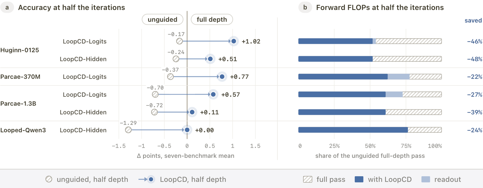
Compute is analytic forward FLOPs for a 512-token prefill, guidance included (reported, Table A9):
| setting | iterations | FLOPs vs full pass | removed |
|---|---|---|---|
| Huginn-0125, logits | 32 → 16 | 0.54 | 46.0% |
| Huginn-0125, hidden states | 32 → 16 | 0.52 | 48.2% |
| Parcae-370M, logits | 8 → 4 | 0.78 | 22.5% |
| Parcae-1.3B, logits | 8 → 4 | 0.73 | 27.3% |
| Parcae-1.3B, hidden states | 8 → 4 | 0.61 | 39.2% |
| Looped-Qwen3, hidden states | 8 → 4 | 0.76 | 23.6% |
No row says 47%. The post's figure sits between Huginn's 46.0% and 48.2%, the two best cases; the paper's range is 22.5% to 48.2%. The ceiling is set by architecture: halving the loops can only remove the loop's share of the pass. Huginn spends most of its FLOPs in the loop, so it approaches half. Looped-Qwen3 has 32 non-looped layers around a 4-layer window, so it cannot.
Three caveats the post dropped, all from the paper itself:
- The half-depth runs are multiple-choice only (reported, Appendix D.1). There is no half-depth AIME number. The 73.33% and the 48.2% never occur in the same run, on the same model, or on the same kind of task.
- Ouro is not in the half-depth study at all. The model behind the AIME number has 4 loops, and the paper does not test it at 2.
- FLOPs, not wall-clock. The paper says its counts "reflect theoretical arithmetic workload rather than end-to-end wall-clock speedups" (reported). Loops run sequentially, so halving them should cut decode latency roughly in proportion on a loop-dominated model (reasoned), but nobody measured it.
What "(almost) free" costs
At full depth, LoopCD-Logits pays for one extra pass through whatever sits after the loop (reported, Table A7):
| model | layers after the loop | LoopCD-Logits FLOPs |
|---|---|---|
| Ouro-1.4B | 0 | 1.019× |
| Ouro-2.6B | 0 | 1.010× |
| Huginn-0125, | 2 | 1.022× |
| Parcae-1.3B | 8 | 1.119× |
| Looped-Qwen3 | 17 | 1.306× |
For Ouro, "almost free" means 1% to 2%: a second norm and vocabulary projection. For Looped-Qwen3 it means 30.6% more compute, because the reference has to run the frozen 17-layer tail. That is why its half-depth result uses LoopCD-Hidden: with the logit form, the readout overhead would exceed the loop savings (the paper's reading of Figure A1). LoopCD-Hidden costs 1.000× everywhere, but a contrast injected before a deep coda gets damped: on Parcae-1.3B's 8-layer coda it keeps roughly 60% of the logit form's multiple-choice gain (0.85 against 1.38 points, reported).
Memory is the cost the paper does not tabulate. LoopCD needs (or ) to still exist when is done: one extra hidden vector per position being decoded (reasoned). At decode time that is small next to the KV cache. In a fused serving kernel that discards intermediate loop states, it is a plumbing change, not a free switch.
The strength knob is narrow for generation
Multiple-choice scoring tolerates a wide band of fixed , peaking near 0.5 (reported, Figure 9). Generation does not: an early token pushed the wrong way changes every token after it. The paper picks of 0.2 to 0.3 for generation, and beyond about 0.6 the curves fall steeply; Ouro-1.4B loses 8 points on GSM8K at and 20 at (reported, Appendix G.1). The adaptive rule widens the safe range, staying positive for caps from 0.5 to 1.0 where fixed strength overshoots (reported). Read the 73.33% with that in mind: it is the adaptive rule at a cap of 1.5 on a model trained, unlike Huginn and Parcae, to make its intermediate loops decodable.
Where it sits among the site's looped-model coverage
This paper is the first in this cluster to ask what to do with a looped model at inference rather than how to train one. Towards looped models done right separates Ouro-style and Huginn-style design choices; the random-init axis it studies is exactly why Huginn's fails as a hidden-state reference here. SMELT and LOOM are about whether more loops pay for their FLOPs at training time, and virtual logic depth about what looping buys at all. LoopCD's half-depth result is a different trade: it does not make loops cheaper, it makes the half of them you kept work harder. (Unrelated despite the name: the site's Contrastive Language Model piece is about contrastive embeddings, not contrastive decoding.)
What I'd take from it
- The amateur problem disappears for looped models. Contrastive decoding always needed a weak model that shares the expert's vocabulary and failure modes. A loop's first pass is that model, and it is already computed (reported mechanism; the contrast form is O'Brien and Lewis's with ).
- Pick the reference by disagreement, not accuracy. The first completed loop wins for logits; noise-initialised models need a post-burn-in state for the hidden form (reported).
- The 73.33% and the 48.2% are separate claims. One is full-depth math with a slightly larger compute bill; the other is half-depth multiple-choice. Neither has a wall-clock measurement or error bars (reported; reasoned on what is absent).
- It is a tie-breaker. It moves 5.8% to 14.9% of ARC-Challenge answers, almost all of them close calls (reported). It cannot rescue a loop that is converging on the wrong answer.
I have not run it. The method is about ten lines on top of any looped model that exposes its per-loop states, and the Ouro checkpoints are public, so the AIME claim is checkable by anyone with a GPU and patience for 480 sampled solutions per AIME year (30 problems, 16 samples each).
- architecture
- OuroForCausalLM
- task
- text-generation
- library
- transformers
- license
- apache-2.0
- safetensors
- 1 shard
- largest file
- 5.34 GB
- files
- 13
- downloads
- 12.2K
- likes
- 158
repo last modified 2026-02-26