Scaling laws in 2026: the line held, the recipe didn't

2026-08-24 · 13 min · scaling-laws · llm · pretraining · inference · explainer

Every retelling of scaling laws has the same shape. A 2020 paper found that model error falls on a straight line as you add compute. A 2022 paper found everyone was building models too big and feeding them too little, and fixed the ratio at about twenty tokens per parameter. Therefore AI progress is predictable, therefore the labs are reading a ruler rather than conjuring miracles.

All of that is true and it stops four years ago. The models shipping this year are trained at 200 tokens per parameter, at 60,000, at 79,000 — and those are not sloppy approximations of twenty. They are a different question being answered. Somewhere between 2022 and now, the thing the industry optimises stopped being the thing Chinchilla optimised, and the most-quoted number in applied scaling became a correct answer that no longer matches the question.

This is the walk from what "loss" actually means, through the two famous results, to the two much less famous ones that added a third axis to the budget.


The line	Kaplan et al., arXiv:2001.08361 · loss falls as a power law in parameters, tokens and compute
The exponents	α_N = 0.076 · α_D = 0.095 · α_C = 0.050 — all small, which is the whole story
The cost	C ≈ 6ND FLOPs · GPT-3 is 3.15×10²³ of them
The reallocation	Hoffmann et al., arXiv:2203.15556 · 400+ models · N and D should scale together, ≈20 tokens/param
What ships now	Llama 3 70B at 214 · Qwen3-0.6B at 60,000 · LFM2.5-350M at 79,096
The functional form	the additive Chinchilla law gets the sign of the allocation trend wrong — covered separately
The third axis	Sardana et al., arXiv:2401.00448 puts serving in the objective; Roberts et al., arXiv:2604.01411 puts inference samples in it
The pace	frontier LLM training compute doubles every ≈5.2 months; cost doubles every ≈7

First, what the word "loss" refers to

Before loss is a dot on a log-log plot it is a surface. Every weight in the network is an axis, the height is how badly the model predicts the next token, and training is a walk downhill.

loss over two filter-normalised directions in weight space — drag to orbitwell-conditioned

roughness0.00

learning rate0.055

step 0 / 220 · height at the walker 0.806

This is what the word loss refers to before anyone plots it against compute: a surface over the weights, and training is a walk downhill on it. Two directions are drawn here because two is what fits on a screen — the real surface has one axis per parameter, so a frontier model’s is a landscape in something like a trillion dimensions.

Turn the roughness up and the walk starts getting caught, which is the picture people reach for when they say optimisation is hard. It is worth being precise about what the scaling laws in the rest of this piece actually claim, because it is not about this picture at all. They say nothing about the route. They predict how low the floor sits once you have finished walking — as a function of how big the model is, how much it read, and how much arithmetic you were willing to buy.

You cannot draw a surface in a trillion dimensions, so the pictures everyone shares are two-dimensional slices. For a long time those pictures were close to meaningless, because a network is invariant to rescaling a filter and its normalisation together — so you can make a minimum look razor-sharp or comfortably wide without changing the network's behaviour at all. Li et al. fixed that with filter normalisation: scale each random direction to match the norm of the filter it perturbs, and two such plots become comparable.

That paper is also the origin of the genre, and its central pair is worth seeing at full size.

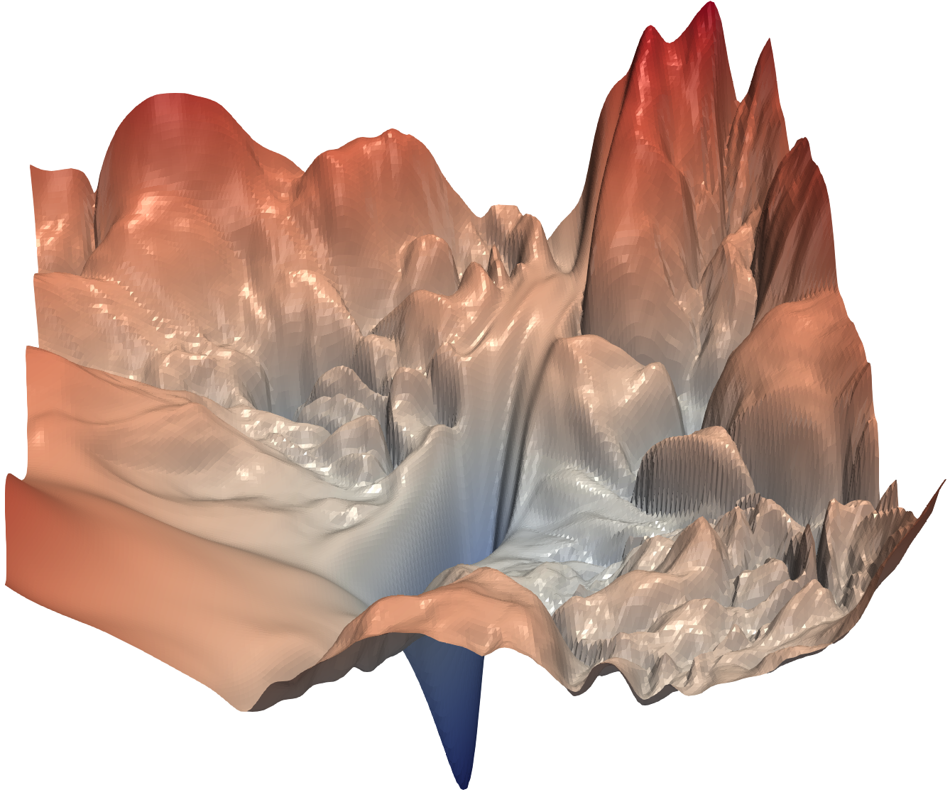
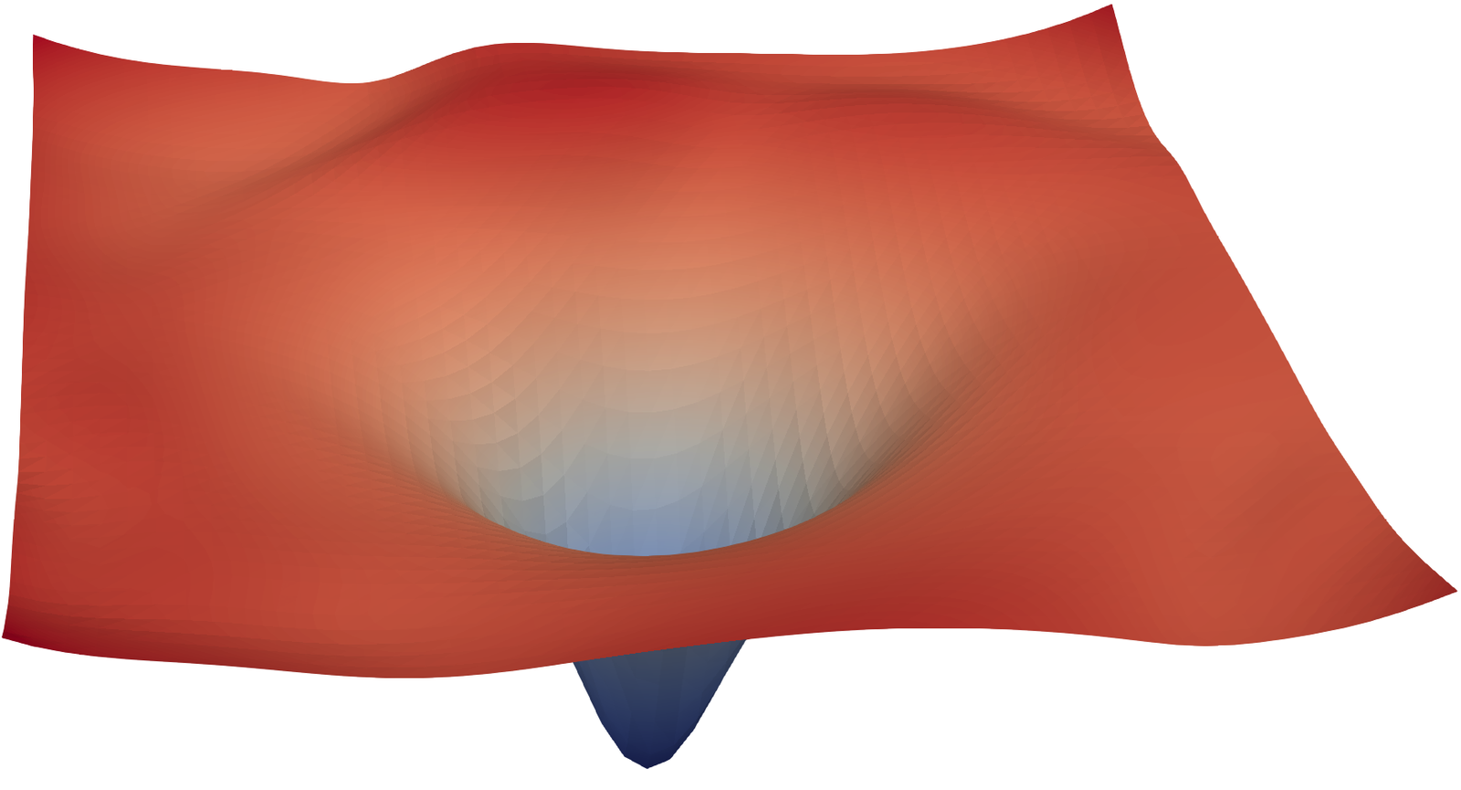
A three-dimensional loss surface rendered in red and white, wildly chaotic: dozens of jagged peaks and ridges surrounding a single narrow blue spike descending to a minimum near the front. — ResNet-56 without skip connections. The surface is not a bowl with some noise on it — it is a mountain range, and the minimum is a needle. (Li et al., arXiv:1712.09913, Figure 1.)

A three-dimensional loss surface rendered in the same red and white palette, this time an almost perfectly smooth wide bowl descending to a single broad basin, with no jagged features anywhere. — The identical network with skip connections added. Same architecture family, same plotting method, same axes. (Li et al., arXiv:1712.09913, Figure 1.)

Here are both shapes as turntables, rendered from scratch for this piece — the chaotic one first, then a well-conditioned bowl with momentum SGD spiralling into the floor.

An animated rotating three-dimensional loss landscape in the viridis colour scheme: chaotic green and yellow ridges surrounding a deep purple crater at the centre, turning slowly through a full revolution.

An animated rotating three-dimensional loss surface: a smooth viridis bowl, purple at the bottom and yellow at the rim, with a pink trajectory that traces a long curve down the wall and spirals into the minimum.

Now the part that matters for everything below, because it is the thing these pictures make people get wrong. Scaling laws say nothing about this surface. They do not describe the route, the roughness, or whether SGD gets stuck. They predict how low the floor sits once the walk is over, as a function of three numbers you choose before it starts.

The line, and why it is shallow

L = (X_c / X)^α — a straight line only once both axes are logarithmicα = 0.050 · one decade buys 10.9%

exponent α0.050

the three reported exponents are 0.050 (compute), 0.076 (parameters), 0.095 (tokens) · drag α higher to see what the curve would look like if scaling were generous

Switch to linear axes and the famous straight line is a disappointing hook that flattens almost at once. That is not a different claim — it is the same numbers, and it is the more honest picture of what buying scale feels like. An exponent near 0.05 means a tenfold increase in compute removes about 11% of the remaining loss, and then you need another tenfold for the next slice.

The line being straight is what makes the spending rational; the line being shallow is what makes it enormous. Both facts come from the same small number, and almost every retelling of scaling laws quotes the first and skips the second.

Kaplan et al. fit three separate power laws, each of the form L = (X_c / X)^α, and the fits hold across more than seven orders of magnitude:

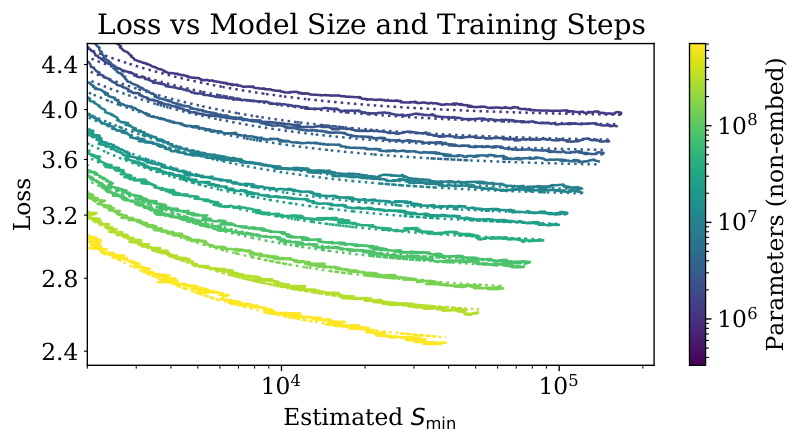
L(N) = \left(\frac{N_c}{N}\right)^{\alpha_N},\quad L(D) = \left(\frac{D_c}{D}\right)^{\alpha_D},\quad L(C) = \left(\frac{C_c}{C}\right)^{\alpha_C}

A log-log plot of test loss against compute in petaflop-days, showing a dense fan of individual training curves in light blue descending to a lower envelope, with a fitted straight power-law line running through the envelope across several orders of magnitude. — Individual training runs, and the straight line their envelope traces. The fit is over the compute-efficient frontier, not over any single run. (Kaplan et al., arXiv:2001.08361.)

The straightness is what makes nine-figure training runs a planning exercise rather than a gamble: fit the line on a ladder of small cheap models, read off where the big one lands, sign the cheque. That part of the standard retelling is exactly right.

The part that usually gets dropped is the size of the exponents. 0.050 for compute means a tenfold increase in arithmetic removes about 11% of the remaining loss. Not 11 points of benchmark score — 11% of what is left of a quantity measured in bits. Flip the interactive above to linear axes and the celebrated straight line becomes a hook that flattens almost immediately, which is a more honest picture of what buying scale feels like from the inside.

The line being straight is what makes the spending rational. The line being shallow is what makes it enormous. Both come from the same small number.

Chinchilla, and the number that outlived it

For two years after Kaplan the field read the paper as advice to spend on parameters. Model size became a leaderboard and MT-NLG reached 530B.

Then DeepMind trained over four hundred models to find where loss actually bottoms out, and found the field had been building models too big and feeding them too little. The compute-optimal recipe scales N and D together, both roughly as the square root of compute — about twenty tokens per parameter.

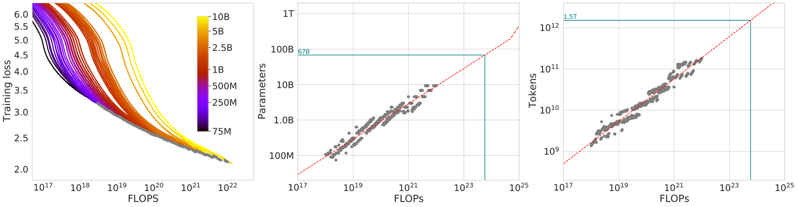
Three panels. Left: many training-loss curves against FLOPs, coloured by model size from 75M to 10B, with grey dots marking the lower envelope. Middle: optimal parameters against FLOPs on log axes, a straight red fit through grey points, extrapolated to 67B at Gopher's budget. Right: the same for optimal tokens, extrapolated to 1.5 trillion. — The envelope in the left panel is what the middle and right panels are fitted to: at each compute budget, which model size and token count sat at the bottom. (Hoffmann et al., arXiv:2203.15556, Figure 3.)

They then proved it in the most humiliating way available: Chinchilla at 70B parameters on 1.4T tokens beat Gopher, a model four times its size, trained on the same compute.

And that is where the popular version of this story stops. Here is what the ratio has actually done since.

tokens per parameter, as actually shippedChinchilla says 20 · 2026 ships 79,096

Chinchilla (2022)70B params · 1.4T tokens · 20 tok/param

the compute-optimal point, and the source of “20”

lifetime FLOPs on serving70%

training, 6ND

5.88×10²³

serving, 2N per token

1.37×10²⁴

lifetime total

1.96×10²⁴

the serving figure is the volume implied by the slider, not a measured one — the point is the shape, not the digits

“Twenty tokens per parameter” is the most-quoted number in applied scaling and it answers a question almost nobody is asking. It is where validation loss bottoms out for a fixed training budget. Push the slider: once most of a model’s lifetime arithmetic is spent answering requests rather than reading, the parameter count is what you pay for forever, and the optimum moves — first to the 100–200 band that inference-aware fits recommend, and then well past it.

The 2026 end of that ladder is not a refinement of Chinchilla. It is three to four orders of magnitude away from it, and it is a deliberate choice rather than a correction: an over-read small model is worse per training FLOP and much cheaper to run for the next two years.

Llama 3 70B trained on 15T tokens — 214 tokens per parameter, more than ten times Chinchilla's recommendation. Qwen3-0.6B reached 60,000. Liquid's LFM2.5-350M put 28 trillion tokens into 354 million parameters, a ratio of about 79,000, roughly four thousand times the number everyone quotes.

None of that is a correction to Chinchilla. Chinchilla is right about the question it asked, which was: for a fixed training budget, where does validation loss bottom out? A lab shipping a model to production is not asking that. It is asking where the lifetime cost bottoms out, and lifetime cost is dominated by inference, where the bill scales with parameters and not at all with how much the model read. Sardana et al. put serving volume into the objective and the optimum moved to roughly 100–200 tokens per parameter. Push the serving slider in the widget above and you can watch the training term stop mattering.

Does intelligence switch on?

Loss is an abstract quantity in bits. What people care about is abilities, and that is where the clean story cracks into the best fight in the field.

Wei et al. reported that certain skills are absent in small models and appear abruptly past a scale threshold — near-random, near-random, then competence. They borrowed the physics word and called it a phase transition.

Schaeffer, Miranda and Koyejo replied that the jump is often an artefact of the yardstick, and won a NeurIPS 2023 best-paper award for it. Grade a task all-or-nothing and per-token skill can climb smoothly the entire time while the score stays pinned at zero, until enough tokens line up at once.

per-token accuracy p, and the all-or-nothing score p^k5% → 50% inside 0.8 orders of magnitude

tokens, all right24

Drag k to 1 and the two curves are the same curve. Drag it to 40 and the score sits at zero for four orders of magnitude and then detonates — while the dashed line, the thing the model is actually getting better at, climbs at exactly the same unremarkable rate the whole way.

Nothing in the model changed between those two pictures. The metric did. That is the Stanford argument in one control, and it won a NeurIPS 2023 best-paper award for it. It does not prove no ability is ever discontinuous — it shows that the standard evidence for discontinuity is also what you would see if nothing discontinuous happened, which means the evidence cannot tell them apart.

The control is the whole argument: the dashed line — what the model is actually getting better at — never does anything interesting, and the solid line detonates. Nothing about the model differs between those two curves. The metric does.

Both sides are right about different things. The underlying loss scales smoothly and predictably; whether a human-meaningful ability appears to jump depends on how harshly you grade it. What the mirage paper establishes is narrower than "emergence isn't real" and sharper: the standard evidence for discontinuity is also exactly what you would see if nothing discontinuous happened, so that evidence cannot distinguish the two.

The third axis

Kaplan and Chinchilla answer the same question in different ways, and they share an assumption that has quietly stopped being true: that a model is finished when training ends. Both optimise a two-way split of a training budget between N and D.

A model that thinks before answering, or that gets sampled twenty times with the best answer kept, is not finished when training ends. Its budget has a third term.

one end-to-end budget, split across parameters, tokens and samplespass@1 = 49.2%

training split → N50%

held for samplingk=1

loss (lower better)

0.658

one sample succeeds

49.2%

any of 1 succeeds

49.2%

training-optimal: split the budget evenly between N and D, one sample

Kaplan and Chinchilla answer the same question — given a training budget, choose N and D — and both treat a model as finished the moment it stops training. That was a fair assumption when a model answered once per question.

It is not one now. Once you are allowed to draw k samples and keep the best, some of the budget should never reach the training run at all — and the model you train with what is left should be smaller and more over-trained than either earlier law would tell you, because a cheap model is what makes drawing twenty samples affordable. The line never broke. It grew an axis, and the axis pushes in the same direction the serving bill was already pushing.

Roberts et al. make this explicit with what they call T² (train-to-test) scaling laws: jointly optimise model size, training tokens and the number of inference samples under one fixed end-to-end budget, with pass@k modelling the test-time half. Their finding is the one that closes the loop with the ladder above — accounting for inference shifts the optimum well into the over-training regime, further than pretraining scaling alone would ever recommend, and the shift survives post-training.

Read the three results together and the trajectory is coherent rather than chaotic:

Kaplan (2020) — for a training budget, loss is predictable. Spend on parameters.
Chinchilla (2022) — for a training budget, spend on parameters and tokens equally. ≈20:1.
Sardana (2024) — for a lifetime budget, serving is paid per parameter. Shrink N, buy D. ≈100–200:1.
Roberts (2026) — for an end-to-end budget including samples, hold compute back for inference, and over-train the smaller model you can now afford.

Each step moves in the same direction, and each one is a consequence of taking a wider slice of the real cost seriously. "Twenty tokens per parameter" is not wrong. It is the answer for a world in which a model is trained once and queried never.

Where this actually stands

Three things are worth stating plainly, because the discourse tends to collapse them.

The line has not broken. Frontier LLM training compute has been doubling roughly every 5.2 months since 2020, about 0.7 orders of magnitude a year, and cost has been doubling every seven to eight months. Those are Epoch AI's numbers and they have not turned over. The commonly-quoted "doubling every six months since 2010" mixes two different series — the 4–5× per year figure covers notable models from 2010 to 2024; the frontier-LLM series is steeper and starts later.

The data is genuinely running out, and that is a real constraint rather than a vibe. Epoch's projection puts the usable stock of public human text at a few hundred trillion tokens and its exhaustion somewhere in the window we are now inside. You cannot keep scaling D indefinitely when D is finite, and a model trained on 28T tokens is already consuming a meaningful fraction of what exists.

The recipe changed and the law did not. Every headline about scaling "hitting a wall" is describing the recipe: a particular allocation of a particular budget, tuned for a world where the training run was the whole cost. The underlying claim — that loss falls predictably in the resources you spend — is doing fine. What changed is which resources count.

The thing worth carrying

The reason scaling laws matter is not that they let a lab predict a benchmark. It is that they turn a question about intelligence into a question about allocation, and allocation questions have answers.

Which is also why the stale number is worth caring about. "Twenty tokens per parameter" spread because it is short, memorable, and sounds like a law of nature. It is none of those things — it is the solution to one optimisation problem, with one budget, under one set of assumptions about what happens after training ends. Every one of those assumptions has since been relaxed by someone, and every relaxation moved the answer by an order of magnitude or more.

The lesson is not that scaling laws are unreliable. It is that a scaling law is a conditional statement, and the conditions have been changing faster than the quotes. If you take one thing from this: before quoting a ratio, ask what budget it was optimising and whether that budget is the one you are actually paying.