2026-10-02 · 16 min · explainer · llm · architecture · transformers · pretraining · scaling-laws
A 1:48 narrated explainer, drawn in code. Every number and picture in it is this article's own; the sources are below.
› transcript
Hi, I'm Corvin. Depth should make a model smarter. This benchmark asks when it actually does. So here is the finding. Whether depth pays off depends almost entirely on the residual connection. Until now, every residual design was tested its own way, so you could not compare them. Fix the parameter count, the data and the recipe. Change only one thing: width versus depth. A token enters at the embedding and climbs the stack. Every block adds into one shared vector. In plain pre-layer-norm, the deep blocks barely change it. They only polish a near-finished vector. That is the curse of depth. Hyper-connections and attention residuals let each block read every earlier layer, so deep blocks keep doing real work. In plain pre-layer-norm, every layer just pours into one stream. Nothing selects an earlier layer. Attention residuals let a layer reach back and read specific earlier outputs, like attention across depth. Hyper-connections route through four streams, strong nearby but still reaching far back. Here is the whole result. Lower is better, and moving left makes the model deeper and narrower. Hyper-connections and attention residuals keep dropping into the deep end. Plain pre-layer-norm turns and rises. When you compose its maps, the constrained version collapses toward a single direction. The fix that gave it stability erased the gain. Depth is a real scaling axis, but only with the right residual stream, and you pay for it in memory. So depth can scale, but only the right residual stream makes the deep layers count. Every source is in the full article. I'm Corvin. Bye!
Four different labs are redesigning the same wire. Kimi K3 ships Attention Residuals, DeepSeek V4 ships mHC, ByteDance proposed Hyper-Connections, and a parallel line of work — LayerNorm Scaling, KEEL, Sandwich-LN, DeepNorm, MoDA — rewrites normalization instead. Every one of them claims to beat the curse of depth: the observation that past some point, stacking more layers stops buying you anything. And every one was trained with its own budget, its own model shape and its own codebase, so you cannot tell from the papers which actually works, or whether the reported gains are about depth at all.
DepthBench (Keyu Wang et al., ELLIS Institute Tübingen and CUHK; @Keyuciallo, 26 Sep 2026) runs the experiment the field skipped. Fix the parameter count. Fix the data. Fix the recipe. Change only the width-depth aspect ratio, , from shallow-and-wide to deep-and-narrow. Then ask: across ten residual designs, when you move capacity out of width and into depth, which designs make the extra layers useful?
The answer is unusually clean. It depends almost entirely on the residual connection. HC and Full AttnRes keep getting better as the model goes deeper-and-narrower, down to an aspect ratio of 9.1 — 640 channels across 70 layers. Pre-LN and its normalization variants get worse. And the two cheaper variants that production systems actually ship, mHC and Block AttnRes, lose the property their parents have.
I read the paper, pulled the released checkpoints' configs off Hugging Face, re-derived the FLOP accounting from its appendix, and read the loss curves off Figure 1. Numbers are labelled Reported (the paper's), Measured (I pulled or computed it from a file) or Reasoned (my arithmetic on the other two).
| What it is | A controlled benchmark: iso-parameter, iso-token width-depth sweep across 10 residual designs |
| Backbone | LLaMA-like, MHA (16 heads), RoPE, RMSNorm, SwiGLU, GPT-NeoX tokenizer, untied embeddings |
| Main sweep | 400M total, 7 shapes, aspect ratio 76.0 (16 layers) down to 9.1 (70 layers) |
| Training | OLMo-core on FineWeb-Edu, 20 tokens/param (8B tokens at 400M, 32B at 1.6B), best LR per architecture |
| Scales | 400M main; 300M iso-backbone; 200M-500M multi-scale; 1.6B validation |
| Winners | HC and Full AttnRes keep improving into the deep end |
| Losers | Pre-LN and norm variants flat or worse; mHC and Block AttnRes lose the gain |
| Artefacts | Code, 162 checkpoints; no licence file in the repo |
The residual stream, and why depth curses it
Start from one layer. A Pre-LN sublayer updates the hidden state as
where is attention or the feed-forward network and is RMSNorm. Unroll it and the top of the network is the input plus a sum of every layer's contribution. The identity term in that sum is the whole reason a deep stack trains at all: the gradient reaching any layer has a path that multiplies by exactly one, so depth alone does not make signals vanish. This is the same single-stream picture that Hyper-Connections widens, and it is the backbone of every Transformer that self-attention runs on.
The cost is that every layer writes into the same vector. Nothing forces a late layer to do anything load-bearing; it can make a small refinement to a representation that is already almost finished. The paper's framing, following Sun et al.'s Curse of Depth and Kimi's Pre-LN dilution, is that this is exactly what happens: as models get deeper, neighbouring deep layers produce more and more similar updates, and the marginal layer stops paying for itself.
The key distinction DepthBench insists on — and it is the one the field keeps blurring — is between trainability and utilization. Pre-LN solved trainability a long time ago; you can optimize a very deep Pre-LN Transformer without it blowing up. That does not mean the depth is used. A design can be perfectly stable and still waste its later layers. So the right question is not "can we train it?" but "does the extra depth translate into effective computation?"
Ten ways to wire a residual
The ten designs fall into four groups by how layer receives information from earlier layers.
- Baseline — Pre-LN. One stream, fixed identity shortcut. Source: only.
- Normalization variants. Same single stream, different normalization. Sandwich-LN (Peri-LN) normalizes before and after each branch. LayerNorm Scaling multiplies the normalized input by , so deeper blocks are dialled down. DeepNorm and KEEL go back to Post-LN but up-scale the residual by a depth-dependent to keep gradients behaved.
- Multi-stream residuals. HC carries parallel residual streams and mixes them with small learned, input-dependent maps. mHC is HC with the mixing matrix pushed onto the Birkhoff polytope by Sinkhorn-Knopp, so it is doubly stochastic and cannot amplify across depth — the stability fix that DeepSeek ships.
- Cross-layer access. Full AttnRes replaces the residual sum with a per-token softmax attention over the embedding and every preceding sublayer output — each layer directly retrieves what it needs. Block AttnRes is the cheaper version Kimi K3 ships: it attends over roughly eight block-level summaries instead of all layers. MoDA gives each layer direct access to earlier layers through depth-wise key-value representations.
That last group is the conceptual cousin of Differential Transformer and the token-mixing redesigns: instead of improving what a layer computes, it changes where a layer reads from. AttnRes is the clearest statement of the idea — a layer at depth gets an attention-weighted read over all earlier sublayer outputs, so early computations have a direct wire to the final prediction rather than surviving only if every intervening layer chose to preserve them.
The fair test: hold the budget, move the shape
Here is why the setup matters more than any single result. Total parameters scale approximately as , where is the layer count, the width and the vocabulary. The dominant term is . So to make a model deeper at a fixed parameter budget you must make it narrower — depth is not a free addition, it is a reallocation. DepthBench treats it as exactly that: pick a budget, then trade width for depth and watch what happens.
The main sweep sits at 400M total parameters across seven shapes, from 1216 wide by 16 layers (aspect ratio 76.0) to 640 wide by 70 layers (aspect ratio 9.1), each within about 2% of the budget (Reported, Table 3). Training is OLMo-core on FineWeb-Edu at 20 tokens per parameter — the Chinchilla ratio — which is 8B tokens at 400M, with a disjoint held-out split for the loss. Crucially, they sweep the learning rate per architecture and report each at its best, so a design cannot lose just because its optimal step size differs: LayerNorm Scaling wants , DeepNorm wants , everything else wants (Reported, Table 4).
I wanted to know the recipe was really what the paper claims, so I pulled the released config for the 32-layer Pre-LN checkpoint. It records d_model 896, n_layers 32, FFN hidden 2400 — exactly Table 3's row — with AdamW at learning rate 0.002, betas (0.9, 0.95), weight decay 0.1, a global batch of 1,048,576 tokens, cosine decay with a 760-step warmup, and a run length of 7,600 steps (Measured, from step7600/config.json). That is B tokens — 20 per parameter, as advertised (Reasoned). The org holds 162 checkpoints in total, the arithmetic spread I would expect from a shape sweep: 30 HC, 24 mHC, 21 Full AttnRes, 15 Block AttnRes, 19 Pre-LN, 14 LNS, and the rest across the norm variants and MoDA, at 200M through 1.6B (Measured, Hugging Face API).
Loss read from DepthBench Figure 1(a); endpoints match the paper's stated numbers. HC and Full AttnRes fall as capacity moves from width into depth (right to left); Pre-LN rises; mHC bottoms out at d/L = 42.7 (L = 24) and Block AttnRes at 56.0 (L = 20), then both turn back up. The cost overlay and the panel are computed from Appendix D's FLOP formula and the KV-cache size: the same depth that buys HC and AttnRes their gains raises prefill FLOPs and more than doubles the KV cache.
The result
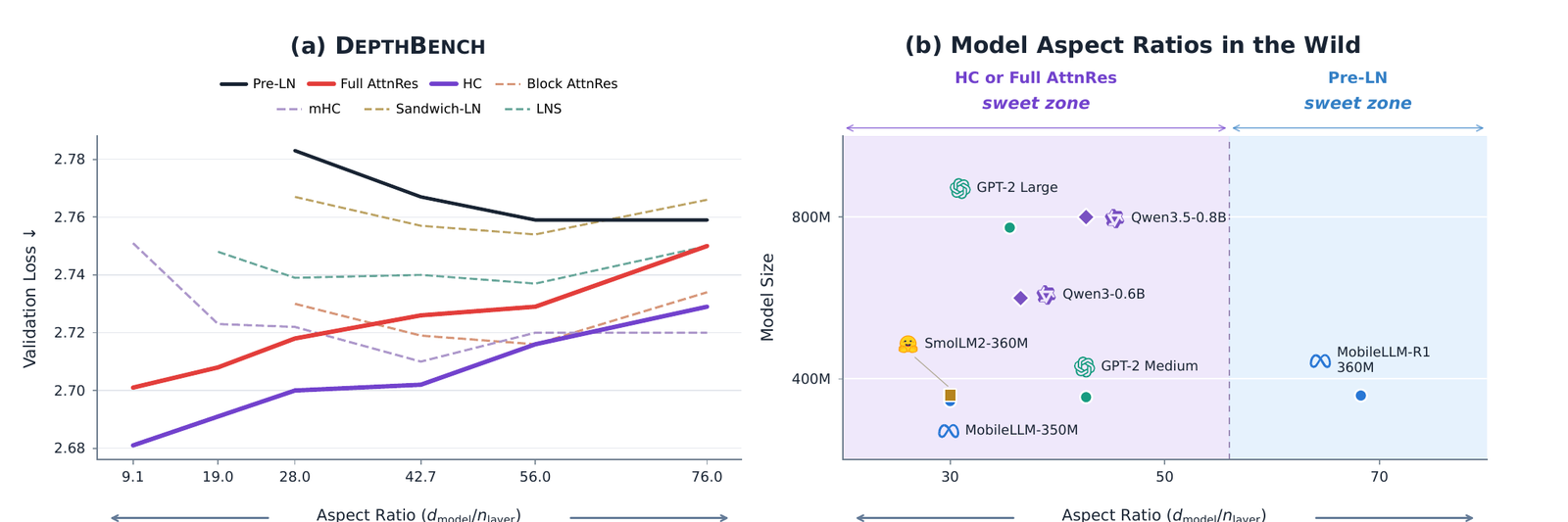
Pre-LN does the opposite of what you would hope. Its validation loss rises monotonically from 2.759 at 16 layers to 2.782 at 32 layers: reallocating parameters from width to depth strictly hurts it, and its optimum stays out at a large aspect ratio (Reported). Sandwich-LN, LNS, DeepNorm, KEEL and MoDA are the same story in weaker form — flat or non-monotonic, with optima at intermediate or shallow shapes.
HC and Full AttnRes invert it. Full AttnRes improves from 2.751 at 16 layers to 2.718 at 32, and keeps going to 2.701 at the extreme 70-layer shape. HC is lower throughout — 2.729 at 16 layers, 2.699 at 32, and 2.681 at aspect ratio 9.1 (Reported, with the deep-end values read off Figure 1). These two designs turn aspect ratio into a scaling dimension you can actually push on. The trend survives the move to 200M-500M, and for Full AttnRes it survives to 1.6B.
The uncomfortable part is what happens to the cheap variants. mHC bottoms out at 24 layers and then climbs; by the deepest shape it is one of the worst designs on the chart. Block AttnRes bottoms out at 20 layers and climbs after that. Both are the versions designed to be affordable — mHC constrains HC's mixing for stability, Block AttnRes collapses AttnRes's all-layer read down to eight blocks — and in both cases the economy measure is exactly what kills the depth scaling.
What "effective depth" actually looks like
The loss curves tell you which designs scale. The analysis tells you why, and it is the most interesting half of the paper. The claim is that effective depth is not "more layers" but structured, differentiated computation across layers — and that you can measure it three ways.
First, representational change. Measuring the angular distance between the hidden state at layer and the state layers later, Pre-LN and the norm variants go smooth: deep layers produce representations that barely differ from their neighbours, converging toward small refinements of one underlying vector. HC and AttnRes stay non-smooth — representations keep changing in a layer-specific, non-uniform way all the way up (Reported).
Second, whether the layers are load-bearing. The paper skips a layer and measures how much that perturbs the update a later layer makes (a causal score), and separately swaps two layers and measures the loss change (a permutation score), restricted to the last three quarters of the network so the always-important first layers do not dominate. For the 32-layer models, only about 1% of Pre-LN's late-layer causal scores are strong, against roughly 16% for Full AttnRes and 7% for HC. Under permutation the gap widens: about 8% for Pre-LN against 46% for Full AttnRes and 35% for HC (Reported). Pre-LN's deep layers are both quiet and interchangeable; AttnRes's and HC's are neither.
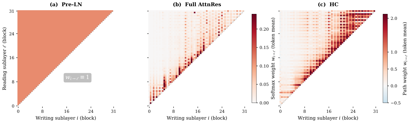
Third, the mechanism itself, in Figure 7. For Pre-LN the cross-depth weight is identically one — it accumulates every update into one stream, which is why its contribution map is a featureless triangle. Full AttnRes instead learns a sparse, non-negative softmax mixture: each layer retrieves specific earlier outputs. HC's effective path is a recursive product of its mixing matrices, strongest locally but still substantial over long ranges. The two winners realize depth in genuinely different ways — AttnRes retrieves stored outputs directly, HC propagates and recombines them through streams — which also shows up in a LogitLens probe: Pre-LN and HC march smoothly toward the final prediction, while Full AttnRes is markedly non-monotonic, consistent with it integrating earlier computations late (Reported).
Why the cheap variants collapse
The two derived designs fail for two different, concrete reasons, and both are worth understanding because both are what shipped.
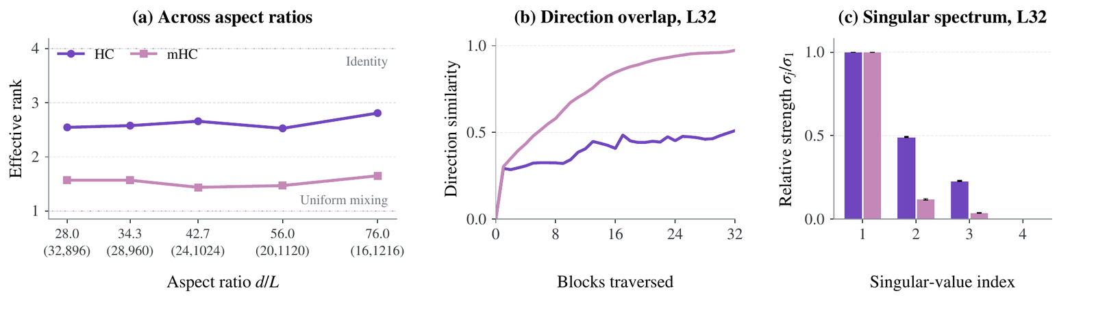
mHC. Composing all of mHC's residual maps along a forward pass gives a product with an effective rank of just 1.44 to 1.65, against 2.53 to 2.81 for HC; at 32 layers mHC's propagated stream directions become nearly collinear (Reported, Figure 10). The cause is the exact property that made mHC stable. A doubly-stochastic matrix has the uniform matrix as a fixed point, and repeated doubly-stochastic mixing contracts toward it — every stream drifts toward the average of all of them. The constraint that stops HC from exploding at 27B parameters is, in the deep-narrow regime, the same force that makes its four streams redundant. This is the irony worth sitting with: mHC was introduced because unconstrained HC gets unstable at scale, and here that very fix is what erases HC's best property.
Block AttnRes fails for a plainer reason. It only saves a new "block" source every few layers, and the paper's own plot of the mixing weights shows that before the first block boundary, the depth-mixing softmax puts essentially zero weight on the running sum — the network drops its own early computation and just re-reads the embedding. That dead segment grows with depth: 2, 5 and 8 layers at 16, 24 and 32 layers, so a full quarter of the 32-layer network cannot benefit from the stacking (Reported). Collapsing AttnRes's all-layer read down to eight blocks is what Kimi K3 does to make it affordable, and it is exactly what spends the depth scaling.
No free lunch
Even at a fixed parameter count, deeper-narrower models are not compute-equivalent, and this is the honest counterweight to the whole result. Since keeps the projection cost () roughly constant while the attention terms () grow, depth quietly shifts the bill toward attention and memory.
I re-derived it from the paper's Appendix D formula. The transformer-body forward FLOPs at a 4096-token prefill rise from 2.98 TFLOP per sequence at aspect ratio 76 to 4.33 TFLOP at aspect ratio 9.1, and the KV cache grows by over the same range (Reasoned, reproducing the paper's reported 3.0-to-4.4 TFLOP and "more than 2x" KV-cache claims). The attention share of the forward pass climbs from about 22% to 35%. The KV cost is identical across all ten designs — it is a property of the shape, not the residual.
The residual designs then add their own overheads on top, and the one that scales best pays the fastest-growing tax. Full AttnRes's depth-mixing cost is roughly — quadratic in depth — so by my accounting it climbs from 0.3% of the base forward pass at 16 layers to 2.3% at 70 (Reasoned). HC and mHC add a flat and respectively, so about 0.5% and 1.3% at 24 layers. On parameters the gaps are small for most designs but not all: against Pre-LN's 405.41M, HC adds 0.3M and AttnRes 0.1M, but mHC adds 4.72M and MoDA a full 48.2M (Reported, Table 6) — so MoDA's "iso-parameter" comparison is quietly spending 12% of the budget on its own machinery.
And measured wall-clock is worse than FLOPs suggest: deeper models run more sequentially, with smaller matmuls and lower hardware utilization. Full AttnRes has the largest peak-memory footprint, and HC posts the highest GPU-hour cost despite a small nominal-FLOP difference (Reported). Depth, done right, shifts the bottleneck from model design to systems design — the same lesson looped models keep teaching, that effective compute and nominal compute are different quantities you have to pay for separately.
What I could and could not check
The configs reproduce the paper's shapes and recipe exactly, the 162 checkpoints are real and named in a way that matches the sweep, and the FLOP and KV claims fall straight out of the appendix's own formulas. What I could not do is re-measure the losses: the checkpoints are OLMo-core distributed-checkpoint shards, not something you load and evaluate in a sandbox, so the loss values here are the paper's own, with the deep-end points read off Figure 1 rather than from a table. The GitHub repository has no licence file at all (Measured, every common filename 404s), which matters if you intend to build on the code.
Two honest caveats on the result itself. HC is the strongest design on the chart but also the least stable: at 500M its largest-aspect-ratio run hits gradient explosion, and at 1.6B it stops showing a clear depth benefit, which the authors attribute to its sensitivity to learning rate — precisely the fragility mHC was built to fix. And the validation-at-scale evidence is three shapes at 1.6B; two or three points cannot tell you whether a trend continues, only that it has not yet broken. The strongest claims here live at 400M, where the sweep is dense.
The take
The useful thing DepthBench settles is that "deep models are better" and "deep models are worse" were both true, and the missing variable was the residual stream. Hold everything else fixed and the width-depth axis splits cleanly: for Pre-LN and its normalization patches it is a dead axis, and for HC and Full AttnRes it is a live one, because those two keep their later layers doing differentiated, order-dependent, causally-consequential work instead of polishing a finished vector.
The sharper lesson is for the cheap variants. mHC and Block AttnRes are the forms that production systems reach for, and both trade away the exact property that made their parents worth copying — mHC's doubly-stochastic constraint collapses its streams toward the mean, and Block AttnRes's block schedule leaves a growing dead zone at the bottom of deep networks. If depth is going to be a scaling axis — and this is the best evidence yet that it is an underused one — the residual that unlocks it is not free, and the affordable approximation may not unlock it at all. That tension, between the design that scales and the design that ships, is where the next round of work has to happen. It is the same frontier the 2026 scaling-law retrospective keeps circling: the line still holds, but the recipe that rides it is still moving.