2026-07-17 · 31 min · mixture-of-experts · linear-attention · kimi · scaling-laws
A 1:45 narrated explainer, drawn in code. Every number and picture in it is this article's own; the sources are below.
› transcript
Hi, I'm Cider! Kimi K3 is the largest open model yet. What's interesting is how its parameters are spent. K3 reworks how information flows three ways: along the sequence, up the layers, and out to its experts. Each makes compute go further. A token climbs ninety-three layers: attention, then a mixture of experts, each time. Three in four attention layers are Kimi Delta Attention. It keeps a fixed-size memory: each token erases a little and writes its own key and value. Every fourth is Gated MLA, full attention for exact recall. None use positional encoding; the delta layers carry order through their decay. Then the experts: sixteen of eight hundred and ninety-six, plus two shared, working in a latent space half the model's width. Attention Residuals let each layer pick from earlier blocks and the embedding, instead of piling everything into one running sum. The router picks one more expert than it needs. That extra score is the cutoff a rival expert had to beat. Each expert's margins, its score minus the cutoff, are binned locally, and one all-reduce sums the bins across the cluster. Its next bias is read straight off a quantile, which hands every expert its target load. No auxiliary loss, no knob. Together, K3 matches K2's validation loss with about two and a half times fewer FLOPs. Parameter count is a spec-sheet figure. More capability per FLOP is the engineering result. To recap: a memory that never grows, residuals that choose, and experts balanced by a quantile. Every source is in the full article. I'm Cider. Bye!
Why read this
Notabletop 60%First-principles tour of K3's KDA, Attention Residuals and 16-of-896 LatentMoE, with the shape checked against the released config.
- Genuinely new idea
- Facts measured from source
- Widely used
LLM architectureNeeds datacenter GPUsSource-availablePractitioner model
How this was scored
- Is it new?
- 3 of 3: Changes how the field does something
- Can I trust it?
- 2 of 3: Measures key facts from files, code or configs
- Can I run it?
- 2 of 3: Open code or weights with real limits
- Will I understand it?
- 2 of 3: Mechanism from first principles with figures
- Can I act on it?
- 1 of 3: General advice
- Will it last?
- 2 of 3: A reference for a year or more
- Does it affect many?
- 2 of 3: A widely used model, tool or lab release
- Only here?
- 1 of 3: Some original analysis
Score 67 of 100, ranked 189 of 577 rated articles. Each question is answered 0–3 by hand, and a 3 is rare. How articles are scored
Moonshot's Kimi K3 is the largest open model anyone has shipped:
2.8 trillion parameters, 104B active per token, a 1-million-token context, natively multimodal. The
weights are now out under the Kimi K3 License, along with a
47-page technical report — so the interesting
claims can finally be checked against a config.json instead of a blog post.
The interesting part is not the parameter count. It is how the parameters are spent. K3 is built on two attention changes — Kimi Delta Attention (KDA) and Attention Residuals (AttnRes) — that rework how information flows across sequence length and across depth, and it scales up MoE sparsity hard: it activates 16 of 896 routed experts per token (plus 2 shared), inside a Stable LatentMoE framework. Together with refined training and data recipes, those structural changes yield a measured 2.5× improvement in overall scaling efficiency over K2. This piece is a first-principles tour of each piece, why it is new, and what a model like this actually costs to build.
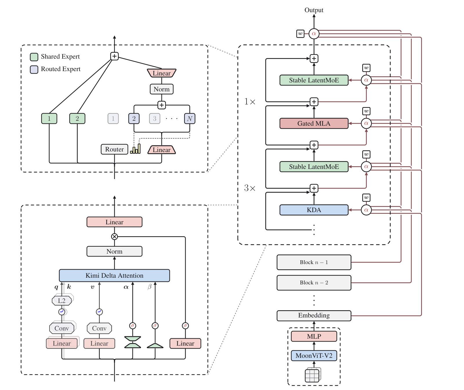
Read the block bottom-to-top: the hidden state passes through the attention sublayer (Gated MLA + KDA), Attention Residuals reach back to earlier depths, and Stable LatentMoE routes the token to 16 of 896 experts before the block emits its output. Four ideas, each doing a specific job. Take them one at a time.
- architecture
- KimiK3ForConditionalGeneration
- task
- image-text-to-text
- library
- transformers
- license
- other
- safetensors
- 96 shards
- largest file
- 16.99 GB
- files
- 119
- downloads
- 1.9M
- likes
- 11.5K
repo last modified 2026-09-02
What the weights actually say
Before the mechanisms, the ground truth. Here is K3's shape as recorded in the released config.json and the report's
model summary:
| Total / activated parameters | 2.78T / 104.2B |
| Layers | 93 (1 dense, 92 MoE) |
| Attention composition | 69 KDA + 24 Gated MLA — 3:1 per block, plus a final global layer |
| Hidden dimension | 7168 · 96 attention heads · head dim 128 |
| Routed experts | 896, 16 active per token, 2 shared |
| Latent MoE dimension | 3584 (half of hidden) · per-expert hidden 3072 |
| MLA compression | kv_lora_rank 512 · q_lora_rank 1536 |
| AttnRes block size | 12 layers (8 blocks, 9 counting the embedding) |
| Positional encoding | none (NoPE) |
| Activation | SiTU-GLU (hidden_act: "situ") |
| Router | sigmoid scoring, noaux_tc — auxiliary-loss-free |
| Vision encoder | MoonViT-V2 · 401M · 27 layers · patch 14 |
| Context / vocabulary | 1,048,576 tokens · 163,840 |
| Quantization | MXFP4 weights, MXFP8 activations (QAT) |
Two of these are worth pausing on. The 3:1 KDA-to-MLA ratio is not approximate — the config lists exactly which
layers are which, and the full-attention layers land on 4, 8, 12, … 92, then 93. The last layer is always global
attention, so whatever the linear layers summarized, the model gets one final unrestricted look at the whole sequence.
And attn_res_block_size: 12 pins down the AttnRes design: 93 layers partitioned into blocks of 12.
Set against K2, the shape of the bet becomes clear:
The official architecture diagram
Kimi Delta Attention: constant-size memory over a million tokens
Ordinary softmax attention keeps a KV cache that grows by one entry per token. At a 1M-token context that cache is the whole ballgame: decoding is memory-bound on a cache that scales with sequence length, and it only gets heavier as the context fills.
KDA is a gated delta-rule linear attention. Instead of a growing cache it keeps a fixed-size recurrent state that each token updates in place: it erases a little of the old state (a gated decay) and writes the new key/value association (the delta rule). The report's exact form applies a channel-wise decay before the delta update:
where is the channel-wise one-step retention factor (the erase, per channel rather than per head) and controls the delta-rule write strength. The state is a fixed matrix — its size does not depend on how many tokens came before. Queries and keys are produced by a short convolution followed by Swish and L2 normalization; values by a short convolution and Swish. Scrub the recurrence and watch the state stay constant-size while a softmax cache piles up:
That constant-size state is what makes a genuine 1M context tractable, and it is why Moonshot reports up to 6.3× faster decoding in million-token contexts. It is not free — a linear-attention state is a lossy summary, not a perfect record, so K3 interleaves KDA with full-attention layers (via Gated MLA) to keep exact recall where it matters. KDA also breaks the assumptions of conventional prefix caching, so Moonshot contributed a KDA implementation to the vLLM community to make serving practical.
FlashKDA: the equation, shipped as a kernel
Moonshot also open-sourced the kernel underneath. FlashKDA (MIT) —
"Flash Kimi Delta Attention" — is a set of CUTLASS kernels for exactly the recurrence above, and its exposed signature
is a direct read-out of that math. The main kernel, flash_kda.fwd, takes query, key and value plus a gate
tensor and beta logits passed through a sigmoid — the gate is , the channel-wise decay; beta is
, the delta-rule write strength — with an optional recurrent state in and out, which is itself: the
fixed-size matrix that is the whole reason a 1M context stays tractable. It also batches variable-length sequences
via cumulative sequence lengths and runs mixed precision (bf16 activations, fp32 params).
FlashKDA needs SM90+ (Hopper and newer), CUDA 12.9+ and PyTorch 2.4+, ships benchmarks for H20 and GB200, and
auto-integrates with the flash-linear-attention library (v0.5.0+) through a chunk_kda op — the same KDA lineage as
the vLLM contribution above, now available as a standalone package rather than only living inside a serving
framework.
NoPE: no positional encoding at all
Here is a detail the weights make unambiguous, and it is one of the quietly radical choices in K3: there is no positional encoding. Not RoPE, not ALiBi, not learned embeddings. K2 used RoPE; K3 applies NoPE to every MLA layer and lets the KDA layers carry position implicitly through their gating and decay — a recurrence is inherently order-sensitive, so position falls out of the mechanism rather than being added to it.
The payoff is at the context frontier. Extending a RoPE model to 1M tokens normally means rescaling the frequency base or applying YaRN-style interpolation, and every such trick is a place quality can quietly degrade. With NoPE there is nothing to rescale: the report says K3 extrapolates directly to 1M-token contexts without any positional-encoding modification. The 3:1 hybrid earns its keep here — KDA supplies position-sensitive, recency-aware mixing, while the NoPE-MLA layers supply unrestricted global content interaction, and the two jobs stay cleanly separated.
Attention Residuals: selective retrieval across depth
The second change is about depth, not length. A plain residual stream compresses all prior information into a single state as it climbs — a bottleneck the report pointedly compares to an RNN over time. Transformers already solved that problem along the sequence axis by replacing recurrence with attention; Attention Residuals applies the same move to depth: each layer selectively retrieves representations from preceding layers rather than accumulating them uniformly. Toggle the two modes and scrub the current layer:
Mechanically, each layer carries a learnable pseudo-query ; the keys and values are the outputs of all earlier layers (plus the token embedding), and attention weights come from a softmax kernel with an RMSNorm inside — the norm stops layers with large-magnitude outputs from dominating the read. Because depth is modest (), the full form is affordable in arithmetic; the real cost is the memory of keeping every layer output alive.
Block AttnRes is the fix, and it is what K3 actually ships. The 93 layers are partitioned into blocks of 12; within a block, layer outputs are summed into one representation, and full attention runs only over the ~8 block-level representations. Memory and cross-stage communication drop from to , and the block structure bounds the inference-time state so inter-block results merge with intra-block partial sums via online softmax. The report notes recovers most of the benefit — which is exactly the 8 blocks of 12 the config encodes.
The payoff Moonshot reports is concrete: about 25% higher training efficiency at under 2% additional cost. That ratio is the tell — a cheap structural change that improves gradient flow and lets the stack go deeper without the usual degradation, which is exactly the kind of lever that compounds into the headline 2.5× scaling number.
Alongside these, the attention sublayer uses Gated MLA — Multi-head Latent Attention with an input-dependent, channel-wise full-rank output gate, letting each token modulate which channels it reads from global attention. The MLP nonlinearity is a Sigmoid Tanh Unit (SiTU-GLU), whose gate branch is a bounded by a constant, so activations cannot blow up. Small pieces, but at 2.8T scale "bounded" is load-bearing.
Stable LatentMoE: 16 of 896, and why that is hard
Here is the aggressive part. K3's feed-forward is a mixture of experts with 896 routed experts, of which only 16 fire for any given token (plus 2 always-on shared experts) — a sparsity of 56. The experts are latent: rather than each selected expert receiving the full 7168-dimensional token, routed experts operate in a compact 3584-wide latent space, half the model width, while the shared experts keep a full-width path. That separation is what makes the expansion affordable — in a conventional MoE, communication and expert-weight traffic grow with routing multiplicity, so going to 16 active experts would be punishing at full width. Scrub a few tokens and watch the selected 16 change:
At this sparsity, two problems that are mild in a denser MoE become first-order. Exploding activations: the routed path composes a down-projection, a gated multi-branch expert FFN, and an up-projection into a chain of nearly four consecutive matmuls — ill-conditioned at 2.8T scale, which is what the normalization and the bounded SiTU-GLU are there to contain. Load balance: balancing nearly a thousand experts per layer exceeds the regime where existing auxiliary-loss-free schemes hold up. If a few experts hog the tokens, the rest never train, and the effective model collapses to something far smaller than 2.8T.
Quantile balancing: no auxiliary loss, no knob
K3 stays auxiliary-loss-free: balancing is done by adding a per-expert bias to the router score before Top- selection, and then omitting that bias from the mixture weights — so it steers dispatch without touching the router's gradients. The standard version nudges by a fixed step in the direction of the load error, which forces a trade-off between slow adaptation and load oscillation.
Quantile Balancing replaces the nudge with a direct solve. Routing runs Top- instead of Top-: the first entries are the routes actually taken, and the -th is the cutoff a competing expert would have had to beat. Each expert's next bias is then read off as a quantile of its margins (score minus cutoff) across the batch — specifically the -quantile — which by construction hands every expert exactly its target load of tokens. No auxiliary loss, no balance coefficient. Drag the quantile and flip to the aux-loss regime to see the imbalance it removes:
At training scale those margins number in the millions and are scattered across ranks, so an exact quantile is not computable. K3 estimates it from a histogram: each rank bins its own margins, a single all-reduce sums the bin counts, and the quantile is recovered from the pooled histogram. Because counts are additive, the estimate reflects the true whole-batch quantile up to the bin width — at a communication cost of a few hundred bins per expert. The bias is frozen at inference.
The systems half matters just as much. K3 uses perfectly balanced expert-parallel training with static shapes and no host synchronization. Variable expert loads normally produce variable tensor shapes, which force recompilation and host-side synchronization that stalls a large cluster. Quantile balancing gives every expert the same load, so the shapes are static, so the expert-parallel pipeline runs without host sync — the difference between 16-of-896 routing being a nice idea and being trainable at 2.8T.
With all four pieces on the table, here is the module-level picture redrawn: the Stable LatentMoE and KDA
blocks in full detail on the left, and on the right the Block Attention Residuals backbone — where each module's
output flows through an α gate that can read every earlier block and the embedding, not just the layer below it.
Read bottom‑to‑top. Kimi K3 stacks a hybrid block — KDA (linear‑time attention), Gated MLA (full attention for exact recall) and Stable LatentMoE (shared + routed experts) — into the residual stream. The twist is Block Attention Residuals: every residual add pulls a gated read (α) off a bus carrying every earlier block’s output, not just the layer below — a learnable skip across the whole depth.
MoonEP: the same static-shapes claim, from the communication side
MoonEP (MIT) is Moonshot's expert-parallel communication library, and it is the static-shapes claim from the quantile-balancing section above, attacked from the other direction. Quantile balancing makes every expert's load equal before dispatch; MoonEP instead guarantees every rank receives exactly tokens — input tokens per rank, routed top- per token — no matter how skewed the actual routing is. The mechanism is a small number of redundant experts, planned online from the current router outputs by a near-optimal GPU planning kernel and prefetched before expert computation runs, with their gradients reduced back to their home ranks on the backward pass. Because those redundant experts absorb whatever skew is left, every rank ends up with an identical, statically-known token count — "statically known shapes eliminate per-layer MoE host synchronization" is not a paraphrase of that claim, it is MoonEP's own description of what it buys. Tokens land directly in their expert-grouped positions on remote ranks through zero-copy buffer views, so only a fixed buffer is needed per layer, with no per-layer host synchronization to stall the pipeline.
Moonshot's own benchmarks against DeepEP v2 on H20 make the case concrete: MoonEP's communication time stays close to flat as imbalance (maxvio) grows, while DeepEP v2 degrades steadily and eventually OOMs under high imbalance — and MoonEP's iteration time holds flat across the same range. It targets NVIDIA GPUs today, with Zhenwu PPU support listed as under review, and credits DeepEP, Echo and UltraEP as inspiration.
Native vision, trained from scratch
K3 is natively multimodal — text, images and video share one backbone and one context, with no post-hoc alignment stage. The notable choice is how the vision tower was trained. Standard practice, including K2.5's own, initializes the encoder from a contrastively pre-trained model like SigLIP. K3 instead trains MoonViT-V2 (401M params, 27 layers, patch 14) entirely from scratch with next-token prediction.
The reason given is stability, and the report shows the receipts: the SigLIP-initialized tower ran persistently higher gradient norms with frequent spikes, while the from-scratch tower stayed smooth. Training under the language-modeling objective also shapes visual features by what the LLM actually needs — fine-grained text and structure — rather than the global semantics a contrastive loss rewards. The conclusion is the interesting bit: MoonViT-V2 matched the SigLIP-initialized baseline on vision evals, so at this scale contrastive pre-training simply was not necessary.
Turning compute into intelligence
Stack it up — KDA's cheap long-context memory, AttnRes's cheap depth, LatentMoE's extreme-but-stable sparsity, plus refined training and data recipes — and the headline is a ~2.5× improvement in overall scaling efficiency over K2. This is not a vibe: it is a fitted scaling-law comparison on held-out out-of-distribution validation data, with hyperparameters (batch size, learning rate, tokens-per-parameter, model shape) re-tuned independently for each family so neither is handicapped by the other's settings.
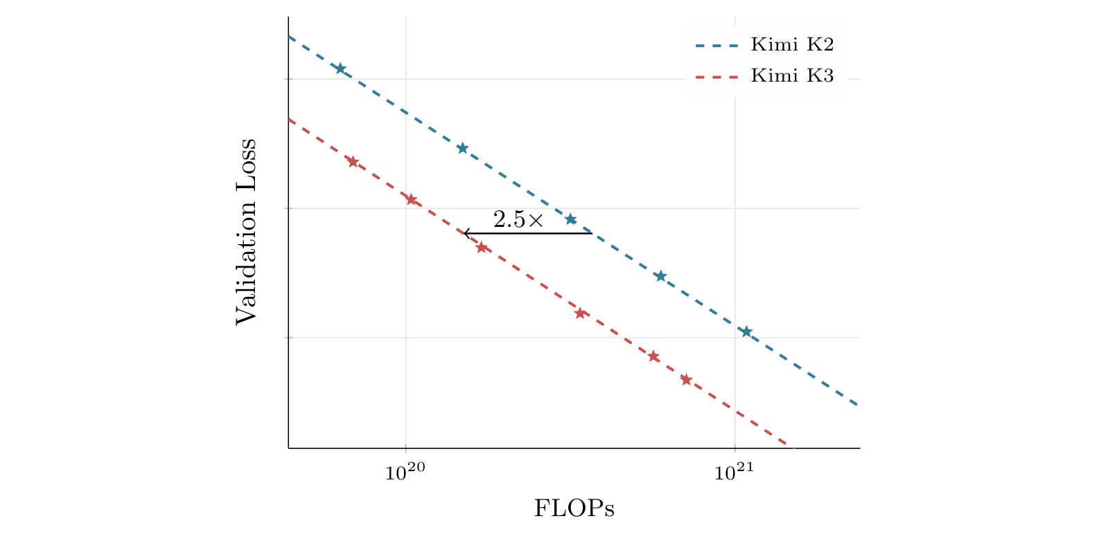
Read the gap horizontally: pick any loss level and the red curve reaches it about 2.5× further left on the FLOPs axis. Drag the capability marker to see the same trade in the other direction:
That is the number that actually matters. "2.8 trillion parameters" is a spec-sheet figure; "2.5× more capability per FLOP" is an engineering result. A side note from the same study, useful to anyone tuning their own runs: under independently optimized hyperparameters, cosine decay consistently beat WSD — the two schedules have very different optimal peak learning rates and batch sizes, so comparisons that share one hyperparameter set tend to be unfair to whichever schedule they fit worse.
What it would take to train it
So what does building a 2.8T-A104B model actually cost? Sparsity still helps: training compute for an MoE scales with the active parameters, not the total, so K3's per-token training FLOPs are those of a ~104B model rather than a 2.8T one. The standard estimate is
with and the number of training tokens. Moonshot still has not published K3's token budget; for reference, K2 was trained on 15.5T tokens. Plug in a frontier-scale budget and pick a cluster:
Three things make that estimate achievable rather than merely large:
- Per-Head Muon. K3 extends the Muon optimizer so that Newton–Schulz orthogonalization is applied to each attention head's momentum block separately rather than to the whole Q/K/V projection. Full-matrix orthogonalization lets large-gradient heads dominate the shared update direction; per-head equalizes the update scale across heads, which improves stability at scale — and is slightly cheaper, since the iterations run on tall thin blocks.
- MXFP4 / MXFP8 quantization-aware training. From the SFT stage onward, K3 trains with MXFP4 expert weights and MXFP8 activations, while attention projections, latent-MoE projections, shared experts and routers stay in higher precision. The model is trained to be low-precision-native, which is why the full 2.8T weights fit in roughly 1.4 TB and why it is servable at all without a quality cliff.
- Static-shape expert parallelism. As above — quantile balancing plus static shapes and no host synchronization is what keeps a large cluster busy instead of stalling on dynamic routing.
The context window is built up rather than trained flat: pre-training starts at 8K and extends to 64K, then the cooldown phase walks 256K → 1M. Concentrating the expensive long-sequence compute into a small slice of the budget is what makes a 1M-token model economical. Length alone does not confer long-range ability, so Moonshot also synthesizes long-context data by permuting and concatenating documents and sub-tasks such that the embedded task can only be solved by attending across the full window — otherwise attention quietly degenerates into local patterns.
Post-training: nine experts, then one
The pre-training story is where the architecture lives, but K3's post-training has a structure worth drawing. It is a three-stage funnel: SFT for a cold-start policy, then RL that trains nine separate experts — three domains crossed with three reasoning-effort levels — then Multi-Teacher On-Policy Distillation to collapse all nine back into the single shipped checkpoint.
The nine are not nine independent runs, and that detail matters. Within a domain, the effort axis is a curriculum over a budget multiplier: each problem x gets a token budget b₀(x) estimated from the cold-start model, and any trajectory whose total exceeds τ · b₀(x) has its task reward overridden to −1 outright. Moonshot trains the max-budget variant first with a large τ, then anneals τ down to obtain the high- and low-effort experts — per domain, with human-in-the-loop tuning of the schedule. For general tasks the budget counts thinking tokens; for agentic tasks it counts cumulative output tokens, reasoning traces and tool-call arguments together.
The collapse back to one model is the part I would have expected to be a distillation loss and is not. MOPD defines a dense per-token reward:
— the stop-gradient log-ratio between the matching teacher and the student, clipped to keep extreme advantages from destabilizing training. Writing it as a reward rather than a loss is what makes it cheap: it drops straight into the existing RL framework, so distillation inherits partial rollout and every other long-horizon optimization built for the RL stage. Moonshot also reports trying finer-grained top-k distillation objectives and seeing no clear advantage in convergence speed or final performance — a negative result that costs nothing to publish and saves someone a month.
A few mechanisms make that work at 1M context:
- Partial rollout. In long-horizon RL, a handful of straggler trajectories can hold up an entire iteration. Generation instead pauses once a fraction of trajectories finish; the rest are enqueued and resumed at the start of the next iteration, backed by persistent sandbox state. That means a single trajectory can span several iterations, so the algorithm has to tolerate badly stale off-policy data — which it does via a per-token regularization that keeps updates in a local neighborhood.
- A white-box harness, not the harness. Training against one fixed agent scaffold teaches the model that scaffold's conventions. Moonshot's RL environment represents a harness as composable modules — tools, system prompts, context management, skills, memories, subagents — and can instantiate Kimi Code, Claude Code, Codex, OpenClaw and Hermes, mixing configurations across task groups so the model generalizes across harnesses rather than overfitting one.
- Deployment-aware training. QAT runs through the entire post-training stage, and during RL the rollout and the training pass share the same quantization scheme — eliminating the train/inference mismatch that usually shows up when a model is quantized after the fact. Separately, K3's pre-trained multi-token-prediction layer is fine-tuned into an EAGLE-3-style draft model for speculative decoding, optimized directly against the acceptance rate rather than a KL surrogate.
Three rewards, three cliffs
The reward functions themselves are the most transferable part of the report, and they share a design decision worth naming.
For non-verifiable general tasks — the ones with no unit test to run — K3 uses an Agentic Generative Reward Model: a tournament-style group reward over binary comparisons, where the judge must follow a mandatory four-step protocol. Read the output; then generate a rubric; then score each candidate against that rubric; then record the scores in a scorepad. Forcing the rubric to be written before the scoring, and forcing the scores to be recorded rather than merely reasoned about, is a cheap structural constraint on a judge that would otherwise be free to justify whatever it preferred.
Bolted onto it is a verbosity guillotine: a candidate whose output exceeds σ · ℓ₀ — where ℓ₀ is the cold-start model's length on that problem — automatically loses the comparison, regardless of content.
The GPU kernel tasks are graded the same way and are more revealing, because the report describes the arms race explicitly. Correctness is a gate: exceed the numerical error threshold and the reward is zero no matter how fast the kernel is. Performance is scored against a human expert's implementation — matching it is worth 0.5, and approaching the hardware roofline pushes the reward toward 1. And then a hacking-detection system penalizes CUDA graph replay, input caching and precision reduction, "continuously extended with new safeguards as new hacking strategies are observed during Kimi K3's development."
That last clause is the honest one. Every one of these three rewards could have been a smooth penalty — subtract something proportional to length, to verbosity, to numerical error — and every one of them is a discontinuity instead. A smooth penalty is an exchange rate, and a policy doing RL will find the price at which a longer answer or a lower-precision kernel is worth paying. A cliff has no exchange rate. The kernel detector is the admission that even that is not sufficient, and that reward design at this scale is a surface you keep patching while something intelligent probes it.
AgentENV: the sandbox layer, and it is open source
The piece that makes all of the above physically possible is the sandbox. Long-horizon agentic RL means running an enormous number of real machines that agents can break, and AgentENV — built by Moonshot with partners, and released under MIT — is the microVM runtime they built for it.
The motivation is refreshingly blunt. Container-based sandboxes were not enough: in early experiments, aggressive agent exploration caused kernel panics and deadlocks. And clamping down is the wrong fix, because hard tasks need a sandbox close to a real machine — agents should be able to mount disks, run containers, even launch VMs. So AgentENV runs each sandbox as an isolated Firecracker microVM, buying isolation and fidelity a container cannot.
On top of that it adds three lifecycle operations tuned specifically for RL:
- Pause / resume. A paused sandbox consumes no memory or CPU. This matters more than it sounds: the sandbox spends as much as 98% of its lifetime just waiting on the model's next inference result. Pausing that window is the difference between renting an idle fleet and not.
- Fork. Branch a new sandbox from the exact state of a running one while the original keeps going — which is how you run a reward judge against a trajectory without any side effects leaking back into it.
- Snapshot. Periodic checkpoints for error recovery.
The engineering is in the latencies: incremental checkpointing saves only pages dirtied since the last checkpoint,
giving 133 ms checkpoint and 49 ms resume. Images use OverlayBD with a custom ublk driver, storage-layer sharing
and P2P transport, so tens of thousands of sandboxes with distinct images launch in under a second; copy-on-write
memory and page-cache tuning push memory overcommit to 6.5× in real workloads.
AgentENV is one of three pieces of that stack Moonshot has now open-sourced: MoonEP (expert-parallel communication, covered under Stable LatentMoE above) and FlashKDA (the attention kernel, covered under Kimi Delta Attention above) are the other two — sandbox, communication and kernel, all MIT-licensed.
The benchmarks
On coding, K3 is a clear #2-or-#3 behind Fable 5 and GPT-5.6 Sol, and ahead of everything else open or closed that Moonshot tested — with a few outright wins.
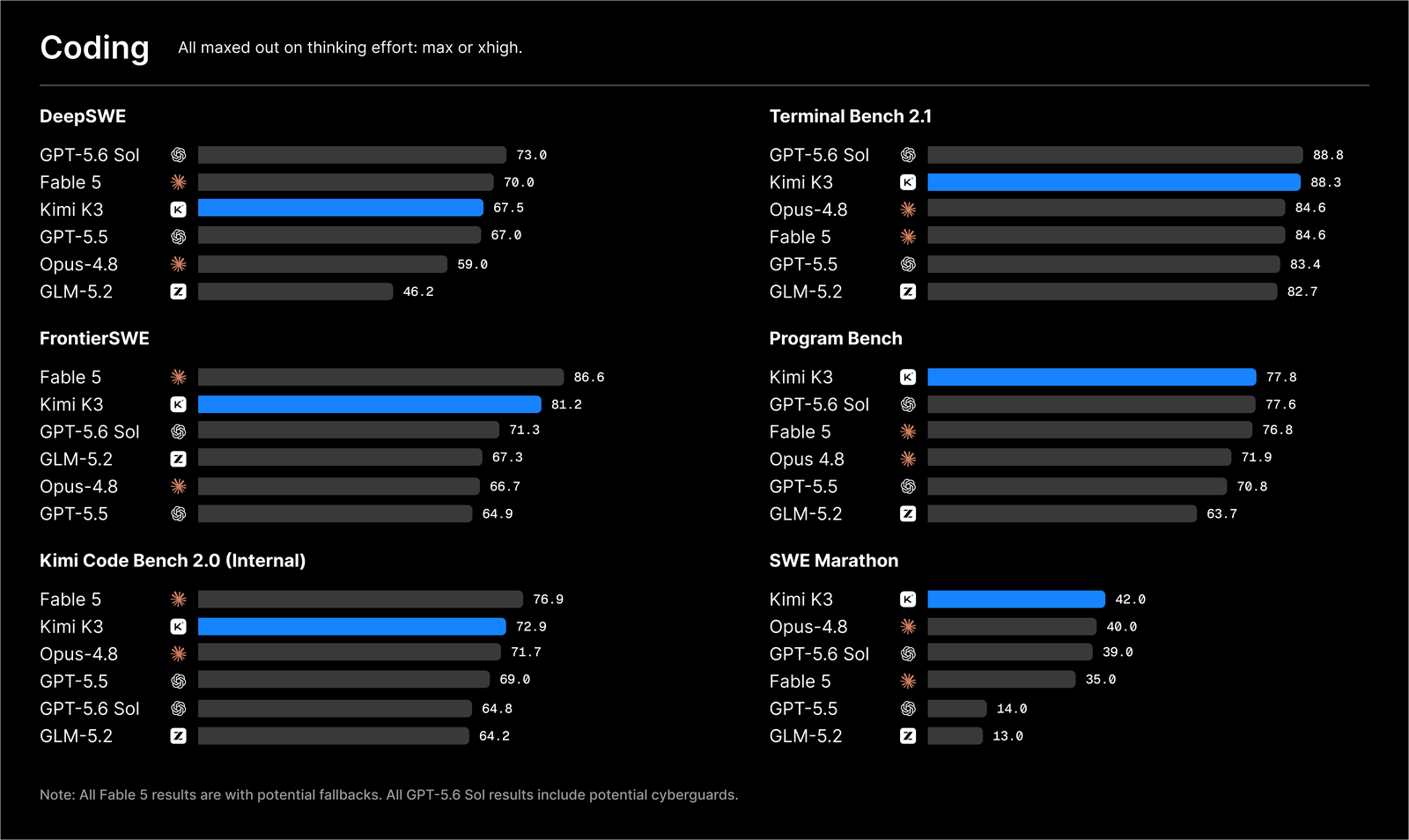
On FrontierSWE it sits second, close behind Fable 5 and well ahead of the rest:
On Terminal Bench 2.1 it is effectively tied for first, and on the long-horizon SWE Marathon and Program Bench it is first outright:
The agentic and visual picture is similar — competitive across the board, and #1 on browsing:
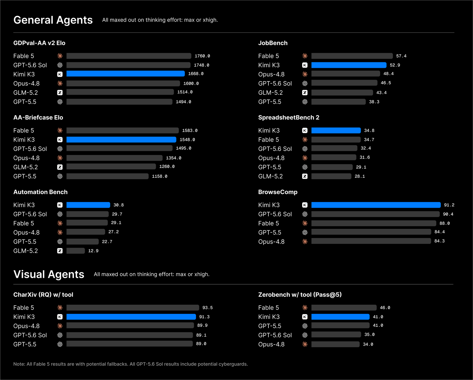
The pattern is consistent: K3 wins where the task is long-horizon and tool-heavy (SWE Marathon, Program Bench, BrowseComp, Automation Bench, SpreadsheetBench 2), and comes second to Fable 5 or GPT-5.6 Sol on the single-shot, knowledge-dense ones (GDPval and AA-Briefcase Elo, DeepSWE).
Independent numbers
The obvious objection to everything above is that it is Moonshot grading its own homework. The report also collects third-party leaderboards, which is the more useful evidence:
| Leaderboard | Kimi K3 | Rank | Best proprietary |
|---|---|---|---|
| Artificial Analysis Intelligence Index v4.1 | 57.1 | #4 / 580 | Fable 5 — 59.9 |
| Vals Index | 74.7 | #2 / 39 | Fable 5 — 75.1 |
| WebDev Arena (Elo) | 1,678 | #1 / 99 | Fable 5 — 1,634 |
| Text Arena (Elo) | 1,486 | #8 / 200 | Fable 5 — 1,507 |
| Agent Arena | 9.1 | #4 / 37 | Fable 5 — 12.7 |
An open model holding #1 on WebDev Arena and #2 on the Vals Index — 0.4 points off Fable 5 — is a materially different claim from a vendor bar chart. Text Arena at #8 is the honest counterweight: general chat preference is not where K3 shines.
What it costs to serve
The sparsity that makes K3 cheap to train makes it cheap to run. API pricing is $0.30 / MTok on cache-hit input, $3.00 / MTok on cache-miss input, and $15.00 / MTok output — and Moonshot reports cache-hit rates above 90% in coding workloads, so the effective input price is closer to the cheap number than the expensive one. MXFP4 weights keep the footprint at ~1.4 TB. The weights ship with deployment recipes for vLLM, SGLang and TokenSpeed.
The report's cost-efficiency comparison is the most quotable result in it:
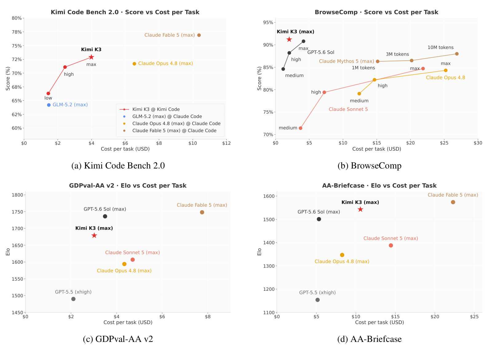
Concretely: on BrowseComp, K3 takes the best score (91.2%) at $2.03 per task — half the cost of GPT-5.6 Sol and an order of magnitude cheaper than the Claude models at max effort. On Kimi Code Bench 2.0 it is 4.0 points behind Fable 5 at 38% of the cost, and at high effort it already matches Opus 4.8's maximum-effort score at roughly a third of the price. On GDPval-AA v2 it is within 50 Elo of GPT-5.6 Sol at 13% lower cost, and 2.6× cheaper than Fable 5.
What it can actually build
The case studies are where the long-horizon claims get concrete, and they are unusually ambitious:
- GPU kernel optimization. Given a sandbox and up to 24 hours per task, K3 cut AttnRes kernel latency from 283.6 ms to 114.4 ms, cut DSA and KDA runtime by 55.1% and 73.6%, and reached over half of peak TFLOPS on MLA — matching Fable 5 and beating Opus 4.8, GPT-5.6 Sol and GPT-5.5. Moonshot notes an early K3 checkpoint was already doing most of their kernel-optimization work during late development.
- A GPU compiler. K3 built MiniTriton, a Triton-like compiler with a
tile-level Python frontend, an MLIR annotation layer and a PTX codegen pipeline, plus a dual-mode tensor library with
reverse-mode autograd and NCCL distributed primitives. On an L20 it beats PyTorch eager and
torch.compilein geometric mean, its from-scratch tensor-core matmul reaches ~90% of the measured machine roof, and it trains a GPT end-to-end with gradients matching torch autograd to within torch's own fp32 rounding error. - A chip. In a single 48-hour autonomous run, K3 designed, optimized and verified an inference-chip prototype (nano-kpu) using open-source EDA tools and the Nangate45 cell library. Inside a 4 mm² budget it closes timing at 100 MHz for an RTL-simulated 8,700+ tokens/s decode, with 1.46M standard cells, 0.277 MiB of SRAM and an INT4 MAC array with fused dequantization.
The take
Strip away the size record and what is genuinely new in K3 is a coherent set of efficiency bets: KDA buys a real 1M context with constant-size memory; NoPE means that context needs no rescaling tricks to reach; AttnRes buys depth almost for free; Stable LatentMoE with Quantile Balancing buys 2.8T of capacity at 104B of active compute and makes that extreme sparsity trainable without an aux-loss knob or host-sync stalls; Per-Head Muon and MXFP4/MXFP8 QAT make the whole thing converge and fit. The sum is the number that matters — ~2.5× more capability per FLOP than K2, measured on fitted scaling curves — delivered in the open at 2.8T.
It does not top the frontier, and it does not pretend to. What it proves is that the gap between open and closed is now measured in scaling efficiency, not in whether an open lab can build at frontier scale at all — and with the weights, the config, and a 47-page report on the table, that claim is now something anyone can go audit.
Sources: the Kimi K3 technical report (architecture, scaling law, post-training, infrastructure, evaluations, case studies), the released model weights and card (config, deployment, license), the AgentENV repository (sandbox runtime), the MoonEP repository (expert-parallel communication), the FlashKDA repository (attention kernels), and the Kimi K3 tech blog (pricing). Figures 3–5 here are the report's Figures 2, 7 and 13, reproduced for commentary. Benchmark numbers are Moonshot's except where marked third-party; the training-cost figures are a first-principles estimate from with clearly labeled assumptions, using K2's 15.5T-token budget as a reference. Interactive diagrams are mine; the routing, loop and cost visuals are illustrative.