2026-10-31 · 20 min · gaussian-splatting · 3d · mesh · robotics

Why read this
Notabletop 60%Rebuilds the wide-angle geometry on the real FIORD lens; checks the 0.60M-Gaussian claim on the released scenes. GOFish itself needs an NVIDIA GPU; not run.
- Original analysis
- A new technique
- Concrete numbers to act on
3D & spatialRuns on a consumer GPUCC-BY-NC-4.0Research paper
How this was scored
- Is it new?
- 2 of 3: A real new idea, method or capability
- Can I trust it?
- 2 of 3: Measures key facts from files, code or configs
- Can I run it?
- 1 of 3: API-only, gated or restrictive licence
- Will I understand it?
- 2 of 3: Mechanism from first principles with figures
- Can I act on it?
- 2 of 3: A concrete recipe, numbers or comparison
- Will it last?
- 1 of 3: Relevant for months
- Does it affect many?
- 1 of 3: A specialist community
- Only here?
- 2 of 3: A teardown or measurement few others did
Score 60 of 100, ranked 381 of 666 rated articles. Each question is answered 0–3 by hand, and a 3 is rare. How articles are scored
The post that sent me here is Allen Tu's: "Introducing GOFish: Full Field-of-View Gaussian Splatting and Mesh Extraction! Reconstruct simulation-ready 3D digital twins directly from fisheye imagery, combining photorealistic #3DGS over the camera's full FoV with a mesh for collisions." The paper is arXiv 2610.37818, v1 of 27 October 2026, by Allen Tu, Meher Gitika Karumuri, Shifan Zhu, Hailing Wang, Yen-Liang Lin, David Held, Matthias Zwicker and Tom Goldstein (Amazon, University of Maryland, UMass Amherst, Northeastern, CMU). It was done during an internship at Amazon. There is a project page, a code repository and a dataset of trained scenes.
The claim is narrow and checkable. Earlier fisheye Gaussian splatting stops short of the lens edge, and surface-reconstruction methods that give you a mesh assume pinhole images. GOFish trains on the fisheye images directly, rasterizes beyond 180°, and pulls a mesh out of the same Gaussians.
What I did: read the whole paper and appendix, read the repository, read the headers of every released scene, and re-implemented the wide-angle geometry in numpy on the real lens calibration that ships with the dataset. What I did not do: run GOFish. It needs an NVIDIA GPU of compute capability 7.0 or newer, a CUDA toolkit and a Slang compiler; this sandbox has none, and it will not execute downloaded code anyway. So no PSNR in this article is mine. Every number is labelled measured (my scripts or my reading of files), reported (the paper's) or reasoned.
A fisheye image is not a pinhole image
A pinhole camera maps a ray at angle θ from the optical axis to image radius . That diverges at 90°. The radial stretch, relative to the lens's own focal length, is : 4× at 60°, 33× at 80°, 132× at 85° and 3,283× at 89° (reasoned, plain arithmetic). A pinhole image of a 200° scene does not exist, so a pinhole splatting rasterizer cannot represent it.
Fisheye lenses spend their pixels differently. The textbook models are
- equidistant, ,
- equisolid, ,
- stereographic, ,
and real lenses are calibrated with a polynomial. The one GOFish uses is OpenCV's fisheye model,
The dataset ships real coefficients. FIORD Hall_In has two cameras on one rig, and their calibrations in cameras.json differ a lot (measured, from the file):
| polynomial stays monotone to | rim at 1,632 px is | |||||
|---|---|---|---|---|---|---|
| camera 1 | 0.0379 | −0.0235 | 0.00284 | −0.000457 | 111.08° | 99.96° |
| camera 2 | 0.0693 | −0.0841 | 0.0427 | −0.00942 | 93.11° | beyond the monotone range |
Camera 1's rim sits at 99.96° from the axis, which is the "200°" in the paper. Camera 2's polynomial folds back at 93.11°: past that angle two different rays land on the same pixel radius, so the calibration stops being a lens. Only 84% of its image disc has a unique ray (measured). This is why the paper does not hard-code a field of view. It lets the calibration say which pixels are valid: rays are unique up to
Try the geometry below. The shaded band is what a 160° crop removes, and the darker one is where camera-space depth is negative.
A 160° crop of a 200° lens removes 36% of the image disc on an equidistant lens and 30% of the solid angle the camera sees (reasoned, formulas in code/exp_fov.py). Pixels more than 90° off the axis are 19% of a 200° disc and 22.9% of a 205° one. For scale, a 120° lens sees a quarter of the sphere, a 160° lens 41.3%, 200° sees 58.7% and 205° sees 60.8%.
For how splat scenes get captured and cleaned in practice before any of this matters, see 3DGS capture pipelines. GOFish is about the rasterizer and the surface, not the capture.
What 3DGUT does, and where it breaks past 90°
Classic 3DGS projects each 3D Gaussian to a 2D one by linearizing the pinhole projection at its mean (the EWA splatting step), then sorts by camera depth and composites. That cannot take a fisheye image. GOFish builds on 3DGUT, which evaluates each Gaussian in 3D along the pixel's own ray. For a ray and Gaussian with mean and covariance ,
That is the exact response of the ray, and it needs no linearization. The rest of the 3DGS pipeline still wants cheap bounds, though. 3DGUT decides which 16×16 tiles a Gaussian touches by projecting seven sigma points through the camera. I read the rule in the repository (gutProjector.cuh, configs/render/3dgut.yaml): the unscented transform has , , , so and the points are the mean and the mean times each column of the covariance factor (with , the rotation-times-scale form the renderer stores), with covariance weights 2 for the centre and 1/6 for the others (read). The projected covariance is dilated by 0.3 px², and the tile extent is standard deviations per axis, capped by a radius built from the larger eigenvalue (read).
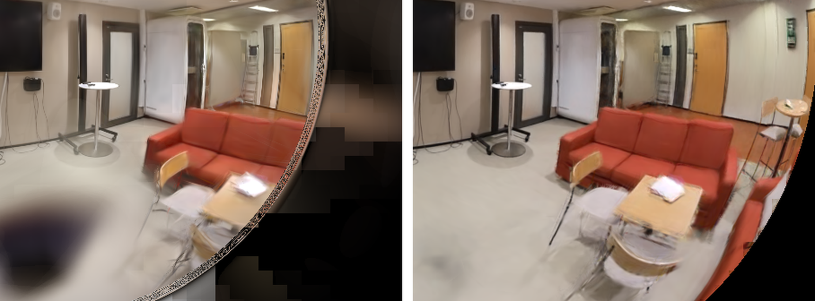
The paper lists three places where this breaks over a wide field of view, shown in its Figure 2:
- The crop. 3DGUT limits the field of view to 160° (an 80° half angle). Rays beyond that are never rendered or supervised.
- The sort. It orders Gaussians by camera-space depth. Depth is , which is negative past 90°, so near-to-far order reverses there.
- The tiles. Tiles come from the projected sigma-point extent, but alpha comes from the exact ray response. A tile whose rays reach the Gaussian can be skipped.
The paper's own comparison of 3DGUT with PPISP (left) against GOFish (right) on a held-out FIORD view shows the first and third failure as a cutoff ring and blocky smears:
What I measured on the real lens
I re-implemented the geometry in numpy (code/fisheye_toys.py) using camera 1's calibration scaled to the 816 px images GOFish trains on, the unscented-transform constants above, and Gaussians with random shapes and orientations at ray angles from 0° to 100°. These are toys: no learned scene, no rendering.
The covariance estimate is not the problem. I compared the projected 2D covariance of a Gaussian from Monte-Carlo sampling through the true lens (40,000 points) against the first-order Jacobian estimate and against the sigma-point estimate. For Gaussians with a standard deviation of 0.05× the viewing distance, both are within about 1% at every angle. For the largest ones I tried (0.2×), the median relative error grows from 3.6% (first order) and 4.3% (sigma points) on the axis to 8.3% and 7.0% at 100°. The area is where they part ways: at 100° the first-order estimate is 14% too small (area ratio 0.86) and the sigma-point estimate is 25% too large (1.25). Neither collapses (measured). The real failures are discrete ones: a crop, a sign, a rectangle.
The rectangle misses a few percent of the tiles. For each Gaussian I computed the exact set of pixels whose ray reaches its support (minimum Mahalanobis distance of at most 3, the cap the paper uses) and compared it with the rectangle the sigma-point rule builds. Explore the table; each cell is 25 Gaussians.
The mean pixel recall is 96% to 100% everywhere, so the rectangle is a decent heuristic. But for the largest Gaussians (σ = 0.2 of the distance), 68% to 92% have at least one supported pixel outside it, and 1.4% to 4.4% of the tiles that hold supported pixels fall outside the tile range (measured). The miss rate is not clearly worse at wide angles in my toy. The paper's visible blocks need a trained scene, where large Gaussians cover poorly observed periphery; my toy only shows that the rectangle is not a bound.
The wide-angle number that does stand out is the last tab. For a Gaussian 90° off the axis, 57% to 100% of the pixels its ray support covers lie more than 80° out. A 160° crop would discard that support entirely (measured).
What GOFish changes
Full field-of-view rasterization
Three changes, one per failure.
Calibration defines the domain. A pixel is valid if it has a unique ray, which gives the above. The same domain is used for rendering, tile admission and meshing.
Complete admission. A Gaussian is drawn in every tile that holds a valid pixel whose ray reaches its effective support. The support radius is . 3DGUT's renderer cutoff is a minimum response of 0.0113, a radius of , so the cap contains it (read, Appendix A.2; the config has the same 0.0113). A tile is rejected only when one of three tests proves that no valid ray in it can reach the Gaussian:
- a domain test (no valid pixel in the tile, or the Gaussian lies beyond the maximum ray angle),
- a Taylor test that encloses the projected support in a rectangle using an interval bound on the projection's Hessian,
- a cone test that bounds all the tile's ray directions in a ball and checks a quadratic.
A failed or inconclusive test keeps the tile. Proposition 1 states that, given a central camera and exact arithmetic, this admits the Gaussian to every tile it can reach; the appendix proves it by contradiction. In practice every bound is rounded outward for floating point. The near-plane cull of 3DGS is dropped.
Sort by ray distance. Admitted Gaussians are ordered per pixel by distance along the ray, using StopThePop's hierarchical sort. The repository's config has the windows: head 4, mid 8, tail 64 (read). That is where the training cost below comes from: the paper's ablation has training 5.6× slower than rendering-only 3DGUT once full-field-of-view rasterization is added (29 to 162 minutes), and the paper says complete admission and per-pixel sorting are the cause. The real-time renderer used for the FPS numbers starts from 3DGUT's projected sigma-point extent instead, with a conservative cone test for Gaussians whose extent is undefined, and trails the complete-admission renderer by only 0.03 dB.
Calibrated Mip Filtering
A pixel averages light over a footprint whose size and shape change across a fisheye image. If the scene does not model that footprint, the exact ray response can only match the blur by baking it into the Gaussians, and then into the mesh. Mip-Splatting separates a view-independent 3D filter from a per-view 2D filter for pinhole cameras. GOFish adapts both to calibrated lenses through the camera Jacobian .
The stored scene gets a 3D filter of radius
added as to the covariance: the finest view that sees the Gaussian sets how much detail the scene may hold. Rendering view adds a footprint that is never stored,
with , and draws the Gaussian with covariance and opacity . Proposition 2 says is the minimum-trace 3D covariance that projects to , and it adds no variance along the viewing ray. I checked the identity numerically on 20,000 random Jacobians: holds to 1.3×10⁻¹³ (measured, code/exp_mip.py).
The 3D filter radius is not constant on a real lens. At one metre of range on camera 1, the smaller singular value of the Jacobian drops from 249 px per metre on the axis to 115 at 100°, because the lens compresses its rim, so grows from 1.80 mm to 3.89 mm (measured).
The part I found most instructive is Proposition 3. Mip-Splatting rescales opacity by the 3D volume ratio . GOFish uses instead, because preserves the integral of the ray-maximum response in the image. The two are related by
with equality exactly when the viewing ray is an eigenvector of . Using would dim Gaussians whose axes are not aligned with the ray, which the paper says darkens surfaces seen at grazing angles. Play with it; the formulas are the paper's, evaluated live:
Over 3,000 random views of each shape with a projected standard deviation of 0.5 to 3 px, the median was 1.00 for round Gaussians (they agree), 0.57 for rods and 0.16 for flat surfel-like Gaussians, with a minimum of 0.065 (measured; the identity held to 7×10⁻⁹, the finite-difference Jacobian's error). Flat, surfel-like Gaussians are what surface-reconstruction methods push towards, which is why I suspect the paper spends a proposition on this (reasoned).
The effect on the scene is on count: the paper reports that removing the filter produces several times more Gaussians with no gain in quality, and that it prevents out-of-memory failures when training and meshing on a 24 GB GPU (reported).
Calibrated densification and the appearance model
Densification normally thresholds a 3D positional gradient, whose meaning in pixels changes with distance and ray angle. GOFish maps each mean's gradient into the calibrated image through , so one threshold serves the whole field of view, and it reuses SOF's densification schedule (reported).
Wide-Angle Appearance Modeling handles the other thing a fisheye does to pixels: the rim goes dark. PPISP models exposure, vignetting, colour and camera response, but its low-order vignetting misses a steep falloff. GOFish multiplies the vignetting by a per-camera : is a nonincreasing radial profile and a low-resolution flat-field map. The released config uses 50 piecewise-linear knots for the profile and a 50×50 grid for the map, both fixed to identity inside half the image radius so they cannot absorb global exposure (read, gofish/appearance/wide_angle.py). is applied after rendering and shared by a camera's views, so it never enters the scene or the mesh. For pinhole cameras it is switched off and the model is PPISP.
The mesh
GOFish uses the same ray-maximum response as Gaussian Opacity Fields. The opacity at a 3D point is the minimum over training views of the alpha accumulated along the ray from that view,
evaluated with stored covariances and opacities, so no per-view footprint or appearance term leaks into it. Points no view observes stay occupied, as in GOF, and full-field-of-view coverage lets peripheral rays fill points that a cropped renderer would leave unobserved. The level set comes from the tetrahedral readout inherited from GOF and SOF. SOF's geometry objective is optional.
What the paper reports
Headline PSNR over each lens's full calibrated field of view (reported, the paper's Table 1):
| FIORD (200°) | FullCircle (205°) | ScanNet++ | |
|---|---|---|---|
| GOFish | 24.36 | 25.47 | 30.17 |
| best prior baseline | 22.08 (DirectFisheye-GS) | 23.50 (3DGRT + PPISP) | 29.71 (3DGRT + PPISP) |
| gain | +2.28 dB | +1.97 dB | +0.46 dB |
| 3DGUT + PPISP, which crops at 160° | 20.18 | 21.45 | 28.93 |
Held-out views from two FIORD scenes, an indoor lounge and a snowy road:
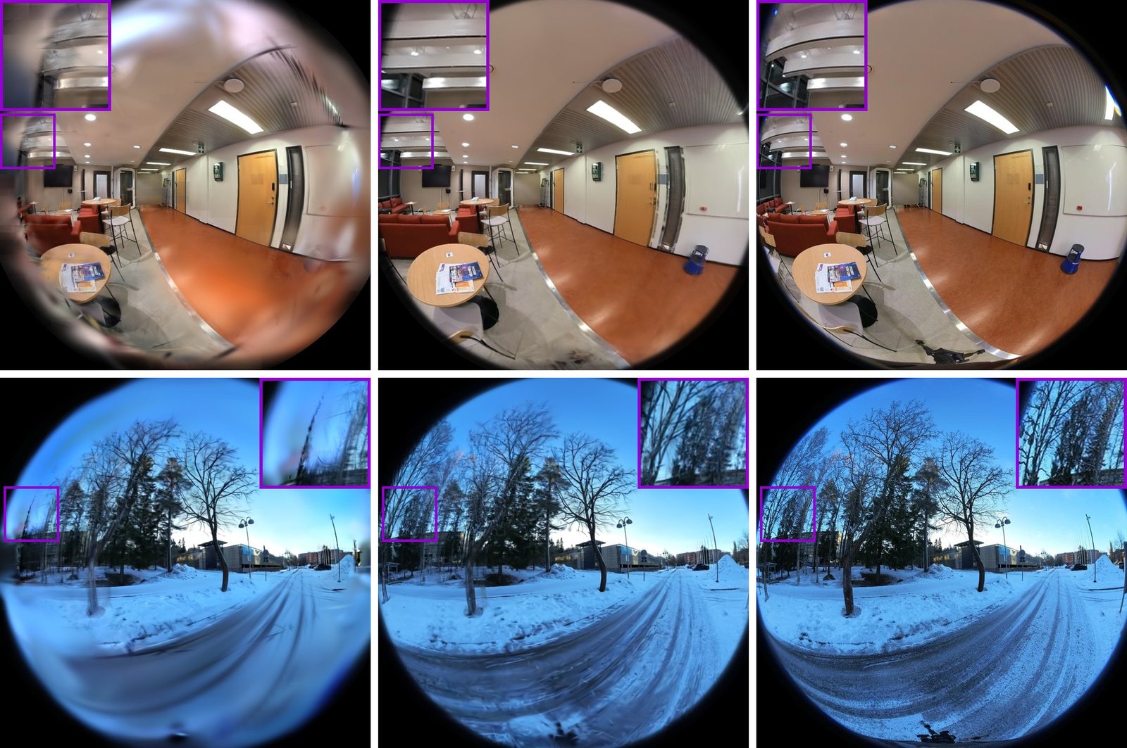
The component analysis (Table 3) is the useful table for a reader who wants to know which piece does what. FIORD, components added cumulatively (reported):
| variant | field of view | PSNR | mesh F-score | training | FPS (A10G) |
|---|---|---|---|---|---|
| GOF | 90° | 17.03 | 0.198 | 104 min | 11.0 |
| 3DGRT + PPISP | full | 18.42 | 0.159 | 108 min | 22.3 |
| 3DGUT + SOF | 160° | 18.46 | 0.168 | 111 min | 17.9 |
| 3DGUT + PPISP | 160° | 20.18 | 0.141 | 29 min | 84.3 |
| + full-FoV rasterization | full | 21.21 | 0.139 | 162 min | 91.1 |
| + calibrated mip filtering | full | 21.19 | 0.240 | 103 min | 81.1 |
| + wide-angle appearance | full | 24.36 | 0.245 | 107 min | 79.3 |
| + geometry objective | full | 24.18 | 0.249 | 116 min | 86.8 |
Read it down the F-score column. Coverage alone does not give a surface: rasterizing the full field of view leaves the F-score at 0.139. Calibrated densification and mip filtering take it to 0.240 with almost no change in PSNR, and the paper attributes 3.6 dB of the 4.0 dB gain inside 3DGUT's own field of view to full-field-of-view rasterization, calibrated densification and calibrated mip filtering together. Wide-angle appearance raises PSNR by 3.17 dB. Ray tracing the full field of view (3DGRT) or bolting SOF's losses onto 3DGUT does not give a competitive mesh. By ray angle, the paper's gain over 3DGUT + PPISP peaks at 5.6 dB in the bin spanning 3DGUT's cutoff on FIORD, and in the outermost bin appearance modelling alone adds 7.9 dB (FIORD) and 1.1 dB (FullCircle): without it, GOFish renders the dark rim too bright and scores below 3DGUT's unrendered black pixels.
The meshes (Table 2): on FIORD, GOFish has the highest recall and F-score of the Gaussian surface methods it compares against (F 0.245, 0.249 with the geometry objective; GOF 0.198, CoMe 0.227, PGSR 0.239, MiLo 0.210), though PGSR has higher precision (0.225 against 0.200). Efficiency, on an A10G: training plus meshing takes 153 minutes against GOF's 208, the real-time renderer reaches 79 FPS against 84 for 3DGUT + PPISP and 22 for 3DGRT + PPISP, and a FIORD scene averages 0.60 million Gaussians against 1.03 million for 3DGUT + PPISP.
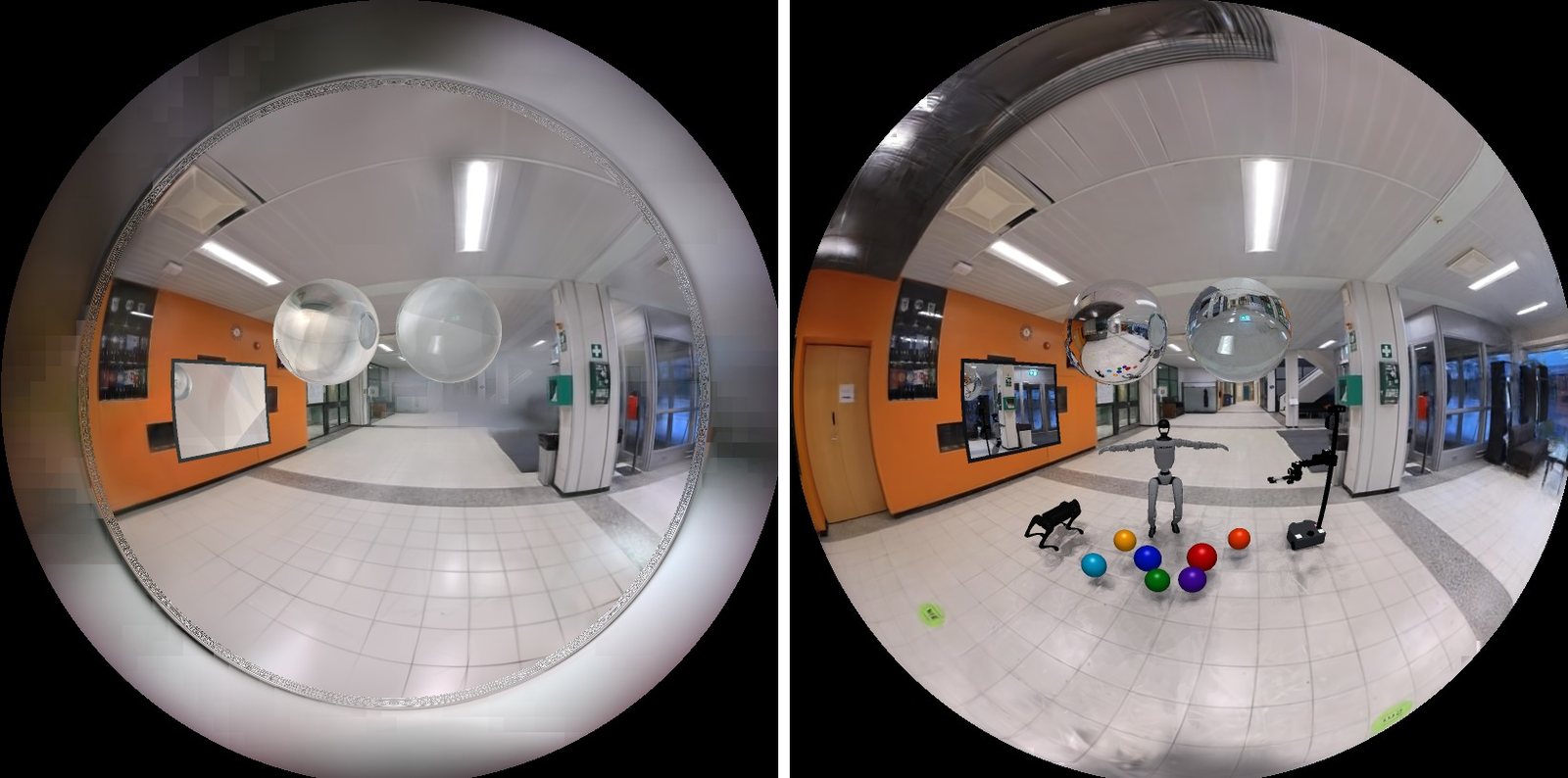
The last capability the paper shows is simulation. A mesh gives you collisions, which a Gaussian scene alone does not:
What the released files show
The dataset card lists the trained scenes: FIORD (200°) and FullCircle (about 205° per lens), each with the Gaussians, the same pipeline with the geometry objective, a mesh and the calibration. It totals 8.25 GB across 201 files and is licensed CC BY-NC 4.0.
I read the first 4 KiB of every point_cloud.ply with an HTTP range request (code/ply_headers.py, nothing else downloaded). The seven FIORD scenes average 598,878 Gaussians, which matches the paper's "about 0.60 million" (measured). Hall_In is the largest at 1,014,691 and MeetingRoom_In the smallest at 427,636. Every file works out to 248.0 bytes per Gaussian (file size over count), 62 float32 values: position, normals, a degree-3 spherical-harmonics colour, opacity, scale and rotation, which is the ordinary 3DGS layout, so existing splat viewers can read the scenes. The per-scene notes say the 3D mip filter is already baked into the stored scales, as the method says it should be.
- license
- CC-BY-NC-4.0
- branch
- main
- tests
- none found
- source
- 2.6 MB
- commit date
- 2026-10-31
by size of tracked source at this commit, file counts in brackets; docs, data and vendored trees excluded
local clone, 2026-10-31 at 1a33e7a — branch, commit, commitDate, fileCount, hasTests, languages, license, licenseFile, shallow
shallow clone: counts describe the pinned tree, not the history
The code is CC BY-NC 4.0, non-commercial, and it keeps third-party licences on parts derived from SOF, StopThePop, CoMe and GOF (non-commercial) and from 3DGRUT, PPISP and Kaolin (Apache-2.0). Installing it takes Python 3.11, a CUDA toolkit, the Slang compiler, and for meshing CGAL plus GOF's tetrahedra-triangulation extension. It builds on 3DGUT/3DGRUT, and the repo has one script per dataset that trains, renders, meshes and evaluates every paper scene (benchmark/fiord.sh and three more). The two components can be used alone, and docs/components.md shows how.
If you want to relate this to the rest of the splat pipeline on this site: SteadySplats attacks sorting, a different part of the renderer, and SOG is about how to store a scene once you have it.
Where it breaks
The paper's own limits, which are real ones:
- It inherits opacity-field behaviour from GOF and SOF: taking a minimum over views can misplace reflective surfaces or carve thin structures, and sparse observations leave holes and overfill. The appendix shows examples of all four.
- Static scenes and central cameras only: moving content, rolling shutter and non-central lenses are out.
- Full-field-of-view coverage cannot recover information lost to sparse sampling or rim attenuation, and reconstruction is sensitive to calibration and pose errors. Among the paper's datasets, only FIORD provides geometry ground truth over the wide periphery, and FullCircle has none at all.
- Training is slower than rendering-only 3DGUT: 107 minutes against 29 on FIORD, though still faster end to end than GOF.
- The FIORD evaluation is not the whole dataset. The authors render seven of its ten scenes, excluding three because their structure-from-motion trajectories are incoherent (one of them also has no LiDAR), and they score Corridor_Out for rendering only because its registration to the LiDAR scan fails.
What I did not check
I did not run GOFish, so none of the PSNR, F-score or timing numbers is a reproduction. My numpy toys use camera 1's calibration and ignore what a trained scene would add: the real 3DGUT crop, its validity rules for sigma points, and tile culling. That is why they measure a rectangle-versus-support mismatch rather than reproduce the cutoff ring. The Monte-Carlo comparison uses Gaussians I generated, not Gaussians from a scene, and 25 to 40 per cell.
The scripts are in public/articles/gofish-fisheye-gaussian-splatting/code/:
python3 exp_fov.py      # lens geometry, real calibrations
python3 exp_cov.py      # Monte-Carlo vs first-order vs sigma-point covariance
python3 exp_tiles.py    # sigma-point rectangle vs exact ray support
python3 exp_mip.py      # footprint identity, Proposition 3, filter radius
python3 ply_headers.py  # Gaussian counts from the released scenes
Sources
- Tu, Karumuri, Zhu, Wang, Lin, Held, Zwicker, Goldstein, GOFish: Full Field-of-View Gaussian Splatting and Mesh Extraction, arXiv 2610.37818, 2026.
- Project page, code and scenes.
- The announcing post: @tuallen_.
- The methods it builds on, as cited by the paper: 3DGUT and 3DGRUT (NVIDIA), Gaussian Opacity Fields, SOF, StopThePop, CoMe, Mip-Splatting, PPISP.