2026-10-31 · 20 min · 3d · gaussian-splatting · gpu

Why read this
Hightop 30%Reads paper, repo and kernel; checks the area proposition; toys split edge, shape and colour; iPad slowdown from raw telemetry. No CUDA run.
- Interactive explanations
- Original analysis
- Runs on a consumer GPU
3D & spatialMITResearch paper
How this was scored
- Is it new?
- 2 of 3: A real new idea, method or capability
- Can I trust it?
- 2 of 3: Measures key facts from files, code or configs
- Can I run it?
- 2 of 3: Open code or weights with real limits
- Will I understand it?
- 3 of 3: Mechanism carried by interactives built from real code or data
- Can I act on it?
- 2 of 3: A concrete recipe, numbers or comparison
- Will it last?
- 1 of 3: Relevant for months
- Does it affect many?
- 1 of 3: A specialist community
- Only here?
- 2 of 3: A teardown or measurement few others did
Score 68 of 100, ranked 174 of 666 rated articles. Each question is answered 0–3 by hand, and a 3 is rare. How articles are scored
The post that sent me here is Prakhar Kaushik's: "Introducing Honeycomb-Surfels (Hexels). High-quality 3D. Less memory. Faster rendering." The paper is arXiv 2610.37668 (Kaushik, Soumava Paul, Alan Yuille, Johns Hopkins). The code is MIT licensed and includes an iPad and iPhone app, Hexel Edge, that trains a scene on the device.
The idea fits in a sentence. Take a 2DGS surfel, a flat disc you intersect with each pixel's ray. Replace its Gaussian falloff with a soft-edged hexagon, and give it a colour that varies linearly across its face instead of one colour. The authors argue that the world is locally flat with smoothly changing colour, so one such patch can stand in for several Gaussians.
I did not train a scene. The CUDA path needs an NVIDIA GPU and the app needs an Apple device; this box has neither, and the sandbox will not run downloaded code anyway. What I did: read the paper's HTML and appendices, read the main repo and its two submodules (the kernel and the viewer), recounted every number I could from files, checked the paper's one theorem numerically, wrote two small CPU experiments, and re-derived one curve from the iPad run's raw CSV. Numbers are measured (mine, from a file or a run of my code), reported (the paper's or the authors' figure, not re-run) or reasoned (my arithmetic on the other two). Related reading on this site: SteadySplats for the renderer side of splatting, and 3D capture pipelines for where a model like this would sit.
A surfel, and what a Gaussian costs it
A 2DGS primitive is a disc in 3D with a centre, two tangent directions and two scales. For a pixel, you intersect the ray with the disc's plane and get local coordinates . The weight is a Gaussian in those coordinates, , multiplied by an opacity, and primitives blend front to back.
A Gaussian never reaches zero. To keep the renderer finite you pick a cut-off, and everything inside it must be visited: the tile assignment, the sort and the blend all pay for the tail. Overlapping tails also mean several primitives share the same pixel. The paper counts this as overdraw and shows it on a poster fitted with 256 primitives (Figure 8, below): about 10 blends per pixel for Gaussians against 2.5 to 2.8 for hexels (reported, read off the figure).
Storage is the other cost. The evaluated 2DGS primitive stores 58 floats; by my count 48 of them are spherical-harmonic colour (3 position, 2 scale, 4 rotation, 1 opacity and 48 colour). That is a lot of memory for a surface whose colour, in many places, is nearly constant or a gentle ramp.
What a hexel is
A hexel keeps 2DGS's frame and ray–plane intersection. Its position , two tangents and two scales place a patch in the world. In the patch's own plane the paper defines a hexagon with one distance function,
so inside, outside and on a regular hexagon with inradius 1. The edge is soft: , with the logistic function and the sharpness the optimiser learns. The hexel contributes alpha , where is its opacity. Colour is a first-order field, : a base RGB and two RGB gradients, in the patch's own coordinates. Compositing is 2DGS's, unchanged.
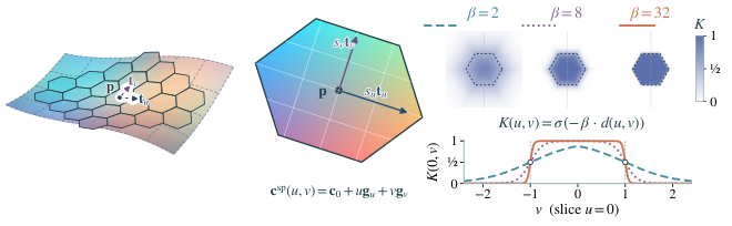
The rasteriser needs to know which pixels a hexel can touch. A contribution below is skipped, and since , that happens where , that is, outside . The bounding circle has radius in the hexel's local units. At the paper's initial that is 1.79 inradii (reasoned, from the paper's Eq. 18 and 19). A Gaussian with equal to that inradius goes on contributing out to 3.33 at full opacity, which is 3.4 times the area. That is a comparison at the same nominal size, not at the same quality; I mention it only because it is the mechanism the authors point to.
Twenty floats
The paper's V1 hexel stores 11 geometry-and-support scalars (3 position, 2 scale, 4 rotation, 1 opacity, 1 sharpness) and 9 colour scalars (a base colour and two gradients): 20 floats, 80 bytes. V2 adds a 3×3 linear view-direction residual (29 floats), and V3 adds degree-3 spherical harmonics (65). The paper gives 58 floats for the 2DGS primitive it evaluates; for 3DGS I used the standard 59, which the paper does not state.
The headline comparison is at matched model memory, so the arithmetic matters: 58 / 20 is 2.9, meaning a V1 model has 2.9 times as many primitives as a 2DGS model of the same size. Whatever the paper's gain is, part of it is simply that. The authors also report a matched-primitive-count comparison (up to +4.74 dB and 2.31 times the frames per second over 2DGS); I come back to those numbers below.
How a pixel finds its
For each pixel the rasteriser needs the intersection of its ray with the hexel's plane. The paper writes the plane's map as a 3×3 matrix from homogeneous local coordinates to the image, takes its rows , and forms , and . Then , with no per-pixel matrix inverse. It skips and anything nearer than 0.2.
That is exact. The paper notes that 3DGS projects a Gaussian with a local affine approximation instead. In a side view the difference is one denominator: the exact local coordinate along a tilted plane is and the affine one drops the term.
The two agree at the centre and drift apart as the plane tilts or the patch grows relative to its distance. That is general to surfels, not special to hexels; I draw it because a hexel's straight edges make the error visible where a Gaussian's blur would hide it.
Why a hexagon: the proposition, checked
Appendix G of the paper gives the argument for the shape. Proposition G.1 says that within a patch, an affine colour field approximates a twice-differentiable target to within , where bounds the second derivative. That defines an ellipse inside which one affine field stays within a tolerance . Proposition G.3 then asks which regular tiling shape, affinely stretched and rotated, covers the most area of that ellipse. The answer is for an -gon, so a hexagon covers times the area of a square and exactly 2 times a triangle.
I checked that numerically. For = 3, 4 and 6 I drew 6,000 random affine maps of a regular -gon, found the smallest disc enclosing each image by brute force, scaled it to unit radius, and compared the area with the closed form. No sample exceeded it (measured: 0 violations in 6,000 for each shape), and the best sampled areas were 1.2990, 2.0000 and 2.5973 against 1.2990, 2.0000 and 2.5981. The ratios come out at 1.299 and 2.000.
Two caveats the paper does not dwell on. The comparison is among shapes that tile the plane. A disc inside the same ellipse covers against the hexagon's 2.598, so the hexagon covers 82.7% of the disc's area; it wins because discs do not tile, not because it covers more than a disc. And the proposition bounds a colour error under a local model; it says nothing about edge sharpness, nothing about how Gaussians overlap, and nothing about optimisation. So I tested those separately.
What a fixed lattice says
The first test removes the optimiser. I tile a image with equal-count lattices of squares, regular hexagons and equilateral triangles, fit each cell by least squares with a constant colour or an affine ramp, and compare PSNR. The lattice scale is bisected so every shape has the same number of cells (border cells otherwise give a hexagonal lattice more cells at the same nominal area). Three synthetic images: a flat-colour poster, the same layout with smooth shading, and a high-frequency texture.
Three things come out (all measured, all on synthetic images, with cell geometry free because the lattice is fixed):
- The colour ramp is the large effect. On the flat poster at 64 cells the ramp adds 3.8 dB for squares (15.80 to 19.59) and 4.1 dB for hexagons (14.97 to 19.03). On the shaded image it adds 4.1 and 4.4. Even at equal stored colour scalars, an affine cell grid of 64 beats a constant one with 192 cells by 1.65 dB (squares) and 1.13 dB (hexagons) on the poster, and by 1.77 and 1.38 dB on the shaded image.
- The shape is within noise. At equal cell count, hexagons and squares differ by between and dB on the poster. With a best-rotation oracle (each shape gets its best of ten lattice angles) the two are level at 64 cells (19.59 each) and at 256 (22.48 against 22.51). Triangles trail squares by up to 1.3 dB at 16 cells. A fixed global lattice does not test what Proposition G.3 is about, which is the best oriented and scaled cell at each location, so this does not contradict it. It does say the effect is not visible when you simply tile.
- On the texture nothing helps. Every shape and colour model sits between 16.6 and 17.6 dB from 16 to 256 cells, against 15.8 dB for one mean colour; the ramp gains 0.05 dB at 64 cells and 0.8 dB at 256. High-frequency content is a different problem, and the paper's own limitations section says as much.
What optimised primitives say
The second test brings the optimiser back. N primitives are placed by image gradient (70%) and uniformly (30%), as in the paper's 2D setup, and trained with Adam for 200 steps, with identical hyperparameters for every kind. Pixels are a normalised blend of all primitives, , which is the paper's 2D renderer without its top-10 cut. Four kinds follow the paper: a Gaussian and a hexagon, each with a constant colour (8 stored scalars) or a linear ramp (14 and 15). Two controls keep the hexagon's sigmoid edge with a fixed and change only the support, to a disc and to a square, so edge sharpness and shape can be told apart. The images are 48 × 48. The main kinds ran on three seeds; the controls ran on two, on the poster and the shaded image only.
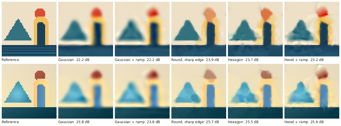
A sharp edge, not six sides. At 32 and 64 primitives on the flat and shaded images, a hexagon with constant colour beats a Gaussian with constant colour by 2.0 and 2.7 dB on the poster and by 2.3 and 3.8 dB on the shaded image (measured, three seeds). That is the size of effect the paper's Figure 8 shows at 256 primitives on its flat image, where constant-colour hexels lead constant-colour Gaussians by 3.0 dB. The round control, with the same sigmoid edge and no corners, does the same: 23.85 and 27.01 dB on the poster against the hexagon's 23.62 and 27.25, and 26.23 and 31.02 on the shaded image against 25.31 and 30.43. Those gaps are inside the seed-to-seed spread, which reaches about a decibel. A square sits 1.2 and 1.6 dB behind the hexagon at 64 primitives, so shape is not irrelevant, but hexagon against disc is not distinguishable here. The strip says why a Gaussian loses: a normalised blend of Gaussians softens every boundary. The paper's Figure 8 has no round, sharp-edged primitive, so as far as I can tell it cannot separate the two explanations; I cannot say whether the answer changes at its scale. The paper does note that "sharper footprints do not by themselves prevent sampling artifacts", which is the caveat to this edge advantage.
The ramp helps when primitives are few. At 8 and 16 primitives the ramp adds 1.0 and 0.9 dB to a Gaussian and 1.4 and 1.1 dB to a hexagon on the poster, and 1.1, 0.9, 1.3 and 1.6 dB on the shaded image. At 32 primitives it is level for a Gaussian (+0.05 and +0.35 dB) and costs a hexagon 0.9 and 0.5 dB; at 64 it costs between 0.6 and 1.5 dB. I read that as an optimisation effect and not a representational one: the ramp adds six or seven scalars to the search and 200 steps do not converge, and the strip's ramp tiles show overshoot streaks. The fixed lattice above shows the representation can carry about 4 dB. But a user training briefly would see this curve, and it is a regime the paper does not report. At equal stored scalars the ramp does not pay for itself here: a hexel with a ramp at 16 primitives (240 scalars) is 1.4 dB behind a constant Gaussian at 32 (256) on both smooth images, and a constant hexagon at 32 beats both.
Texture defeats everyone. On the texture image every kind sits within a few tenths of 16.4 dB up to 32 primitives, which is under a decibel above the 15.6 dB of painting the whole image its mean colour (measured). At 64 primitives the hexel with a ramp reaches 17.05 and the constant hexagon 16.69. The paper's limitations paragraph says it directly: a first-order colour model cannot represent arbitrary texture within one primitive, and high-frequency appearance needs smaller primitives or a richer model.
My first run was wrong in a way worth reporting. I had parameterised the ramp in image units, so with Adam's step of 0.01 the coefficients could not reach useful values, and the ramp looked useless at every size. The paper's Eq. 4 uses local, scale-normalised coordinates . I switched to that, reran the linear kinds, and everything above is the second version; the first version's linear rows are kept in the raw file marked as such and are not used.
What the paper reports
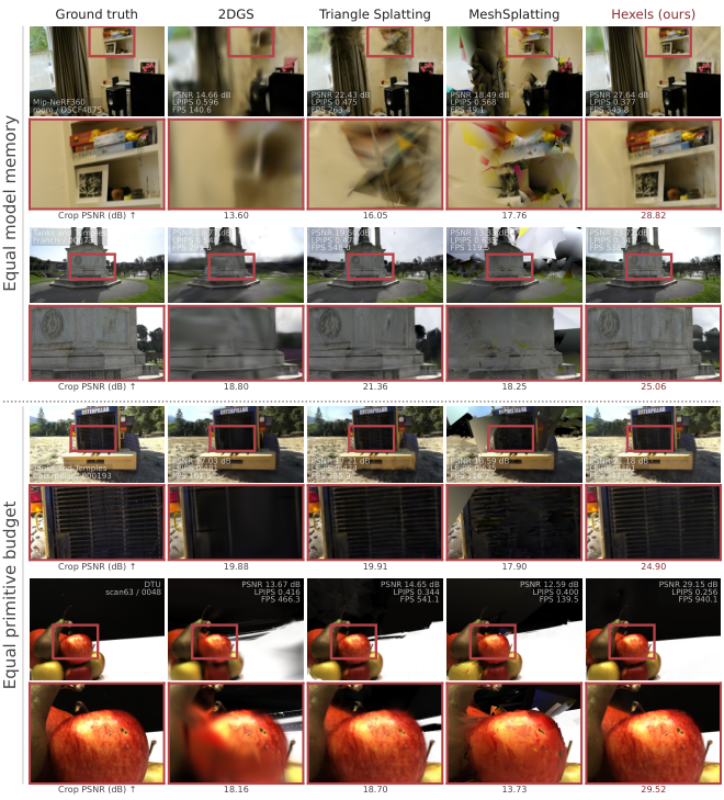
I did not re-run any of this. Table 2 compares methods at matched model memory over 34 scenes. Three rows carry the story:
| Mean over scenes | 2DGS | Triangle Splatting | Hexels V1 |
|---|---|---|---|
| Tanks and Temples (10): PSNR / VRAM / FPS | 18.52 / 1.37 GiB / 284.5 | 21.35 / 0.74 / 495.2 | 23.05 / 0.56 / 438.4 |
| Mip-NeRF 360 (9): PSNR / VRAM / FPS | 17.82 / 3.24 / 201.2 | 22.36 / 1.12 / 312.7 | 24.82 / 0.90 / 377.8 |
| DTU (15): PSNR / VRAM / FPS | 21.56 / 0.68 / 478.0 | 26.04 / 0.69 / 517.5 | 28.94 / 0.55 / 830.8 |
The abstract's "+4.53 to +7.38 dB over memory-matched 2DGS" checks out against the table: 23.05 − 18.52 is 4.53, 24.82 − 17.82 is 7.00, and 28.94 − 21.56 is 7.38 (reasoned, from the paper's own table). The teaser's 5.51 times less peak VRAM (0.88 against 4.88 GiB) is consistent with the rounded values: 4.88 / 0.88 is 5.55. The frames per second advantage over 2DGS is 1.54 to 1.88 times at matched memory.
Not every column favours hexels, and the paper shows it. Training time is not lower: 13.3 minutes against 10.6 on Tanks and Temples, and 24.2 against 20.0 on Mip-NeRF 360, with a tie on DTU (both 8.4). Triangle Splatting trains faster than hexels on all three. The claim is about memory and quality, not speed of training. On 2D images the claim is better quantified: 35.82 against 33.16 dB on the 45-image Image-GS benchmark at 10,000 primitives, in 157.07 against 238.40 seconds, which is 34.1% less time and matches the post. For surfaces, the paper reports 28.9% lower Chamfer error than memory-matched 2DGS across 15 DTU scans, and an F1 of 34.38% against 31.72% on six Tanks and Temples scenes.
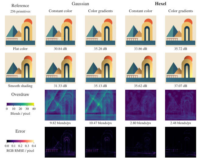
This figure is the cleanest piece of evidence for the shape claim, and it is also what my toy cannot reproduce at its scale: the paper's 256 primitives on a large image is a different regime from my 8 to 64 on a 48-pixel one.
What the release contains
The main repository is MIT. Its THIRD_PARTY.md is worth reading: the vendored baselines (Image-GS, 2DGS, 3DGS, Convex and Triangle Splatting, BBSplat and others) keep their own licences, and the Gaussian-Splatting licence limits those files to research and evaluation. The CUDA kernel and the WebGL viewer live in two separate submodule repositories, both MIT.
I counted lines by script. The Python package hexels/ is 17,259 lines in 30 files, tests/ is 10,216 in 26 files and scripts/ is 8,710 in 47. Hexel Edge is 5,177 lines of Swift in 26 files and one 365-line Metal file. The kernel repository's CUDA source is dominated by a 5,744-line 3D forward file.
The kernel matches the paper where I could compare. It defines the hexagon as the maximum of three half-plane distances, the circumradius constant , for the cut-off, the 0.99 alpha clamp and the threshold. It also has things the paper's main text does not describe:
- A different softness per edge orientation. The model class has a
softness_modethat is"iso"by default and"aniso"for three softness values per primitive, one for each of the hexagon's edge orientations. - An optional screen-space prefilter. When a flag is on, the kernel also computes a Gaussian in screen space (about 0.7 pixel wide, from a constant
kFilterInvSquare = 2) and uses it in place of the hexagon's alpha wherever it is larger, which looks like a guard against primitives smaller than a pixel (my reading). The option,prefilter_edge_on, defaults to off. - More parameters than V1 to V3. The model allocates a 3×3 quadratic colour term, a specular term, and a mechanism for attaching child primitives to parents. The learning rate for the quadratic term defaults to unset and children are disabled by default, so I read these as research options, not part of the released models (inferred: I did not trace every path).
None of this is a criticism. It is a reminder that the paper's V1 is a subset of what the code can do.
On the iPad
Hexel Edge is the part of the release I can say the most about, because the authors publish raw files: a JSON summary, a 34-row quality curve and a 233-row telemetry CSV. The run trains DTU scan24 on a 12.9-inch iPad Pro with an M2, offline and unplugged, for 20 minutes: 6,598 fixed V1 hexels, 42 training and 6 reserved views at 640 × 480, 32,920 updates, 25.21 dB on the reserved views (reported). The authors state the limits themselves: it is one scene, and the reserved views were reused when choosing the recipe, so it is a development number and not a blind benchmark.
I checked what I could. Ledger arithmetic: 6,598 hexels at 80 bytes is 0.50 MiB, and with gradients and two Adam moments about 2.0 MiB; the telemetry's GPU allocation is 2.44 MiB, constant over the run. The peak process footprint is 64.9 MiB, so the parameters are under 1% of it and the whole training state about a thirtieth; the rest is the app, the images and the system (reasoned).
One thing is not in the README. The telemetry's step time is a running mean, which drifts from 23.4 to 35.4 ms. Rebuilding the cumulative update time from it (the mean times the number of updates after the first 40) reproduces the JSON's 1,164.112 seconds exactly, so the reconstruction is consistent. From it, the first 7,000 updates took 28.2 ms each and the last 3,600 took 43.0 ms (measured, my derivation): throughput fell from 35.5 to 23.2 updates per second over the 20 minutes, about 1.5 times slower per update, while the OS reported a nominal thermal state in all 233 samples. The authors say GPU clocks and temperature were not measured, so I cannot name the cause. It is a reminder that a 20-minute figure on a tablet is not a steady-state figure.
The README's status table is candid about scope: V1 hexels in FP32 with a fixed population are implemented; V2 and V3, densification, standalone SfM, quantisation and 2D fitting in the app are not. The iPhone build has been tested only in the simulator.
What I did not do
I did not run the CUDA kernel, train a scene or reproduce any table. The toys are small: 48-pixel images, up to 64 primitives, 200 Adam steps, a dense normalised blend instead of the paper's top-, one set of hyperparameters for every kind. The absolute PSNRs are low because nothing converged; only gaps at the same budget mean anything. I did not tune per kind, and I did not use a photograph, because none is available offline and I would not fetch one I could not license.
What would settle the open questions: a run of the released trainer on one Mip-NeRF 360 scene at matched memory against 2DGS, with the shape and sharpness ablated the way my controls do; the paper's own Figure 8 repeated with a round, sharp-edged control; and a longer iPad run with GPU clocks logged.
Sources
- Kaushik, Paul, Yuille, Honeycomb-Surfels: Compact Hexagonal Primitives for Efficient Scene Rendering and Reconstruction, arXiv 2610.37668 (CC BY 4.0).
- honeycomb-surfels/hexels at 698d1af, with hexel-kernel at 3af3220 and hexel-viewer at ff497d4.
- Project page and the announcement post.
- Hexel Edge results:
hexel_edge/results/dtu_scan24_ipad.json,dtu_scan24_quality.csvanddtu_scan24_telemetry.csvin the main repository. - Experiment scripts and raw results:
public/articles/hexels/code/(tilings.py,primitives.py,prop_g3.py,grid.jsonl,tilings.json).
- license
- MIT
- branch
- main
- tests
- 34 files
- source
- 2.1 MB
- commit date
- 2026-10-29
by size of tracked source at this commit, file counts in brackets; docs, data and vendored trees excluded
local clone, 2026-10-31 at 698d1af — branch, commit, commitDate, fileCount, hasTests, languages, license, licenseFile, shallow, testFileCount
shallow clone: counts describe the pinned tree, not the history