2026-10-31 · 22 min · nerf · cuda · kernel-fusion · hash-grids · novel-view-synthesis

Why read this
Notabletop 60%Featurizer, loss and MLP kernels read; layout and byte counts computed from the config; two labelled toys. No GPU, so no timings.
- Interactive explanations
- Original analysis
- Runs on a consumer GPU
3D & spatialMITPractitioner teardown
How this was scored
- Is it new?
- 1 of 3: An incremental tweak
- Can I trust it?
- 2 of 3: Measures key facts from files, code or configs
- Can I run it?
- 2 of 3: Open code or weights with real limits
- Will I understand it?
- 3 of 3: Mechanism carried by interactives built from real code or data
- Can I act on it?
- 2 of 3: A concrete recipe, numbers or comparison
- Will it last?
- 2 of 3: A reference for a year or more
- Does it affect many?
- 1 of 3: A specialist community
- Only here?
- 2 of 3: A teardown or measurement few others did
Score 66 of 100, ranked 233 of 666 rated articles. Each question is answered 0–3 by hand, and a 3 is rare. How articles are scored
On 30 October a researcher posted that they had written a fully fused Zip-NeRF "with Opus": 36 minutes of training, 300 ms per megapixel on an RTX 5090, "same quality as the official code (~6-7x/10x faster)". The repository is fhahlbohm/fused-zipnerf, MIT-licensed, two commits old, small enough to read in an afternoon. I read the Python in full and the featurizer, the loss kernel and the MLP chain line by line; the optimizer and the ray-generation and compositing helpers I read for structure.
The short version. The design is what the README says it is: hand-written CUDA kernels with analytic gradients, no autograd and no tiny-cuda-nn, and the part that makes it fast is one thread per ray interval doing the hash-grid lookups, the downweighting and the small density network without writing anything in between. The numbers in the post are the README's, and I could not reproduce them, because I had no GPU. Two of its ratios do not follow from the README's own figures, and the repository does not mention the model that wrote it.
Every claim below carries a label. Read means I read it in the source at the commit named at the end. Computed means I derived it by script from the repository's own config. Toy means a small experiment of mine on a CPU, built from the repo's formulas, that illustrates a mechanism and predicts no GPU speed. Reported means the README or a paper says it and I did not reproduce it.
- license
- MIT
- branch
- main
- tests
- none found
- source
- 180.1 kB
- commit date
- 2026-10-31
by size of tracked source at this commit, file counts in brackets; docs, data and vendored trees excluded
local clone, 2026-10-31 at b240dad — branch, commit, commitDate, fileCount, hasTests, languages, license, licenseFile, shallow
shallow clone: counts describe the pinned tree, not the history
What was released
Ten Python files with 600 lines, and nine .cu, three .cuh and six .h files with 2,815 lines (computed). A config for the garden scene of the Mip-NeRF 360 dataset. A README, an MIT licence and a setup.py that builds the ahead-of-time kernels. The repository has no test files, no .github directory and no workflow files: a find for any of them comes back empty (computed). It is two commits: "Initial commit" on 30 October and "Add median depth rendering" on 31 October. It is an extension for the NeRFICG research framework, which supplies the dataset loader, the camera classes and the training loop, so it does not run on its own.
It reimplements Zip-NeRF (Barron et al., ICCV 2023), following the official JAX code. The README's own summary of what it replaces is exact: the official JAX and autograd pipeline becomes "hand-written CUDA kernels and analytic gradients, without tiny-cuda-nn or PyTorch autograd".
Zip-NeRF on one page
You need the model to read the kernels, so here is the part of the paper that matters, as the paper tells it (reported). A hash-grid NeRF such as Instant-NGP looks up features at a point. A pixel is not a point. It is a cone, and the stretch of ray between two samples is a conical frustum. Querying the grid at the frustum's centre treats a footprint that may cover many cells as if it were infinitely small, and the finest levels, which cannot resolve anything that large, return confident noise. That is aliasing, and it shows up as shimmer and as thin structures that appear and vanish as the camera moves.
Zip-NeRF's answer has two halves. First, multisample each frustum with six points on a hexagon, rotated around the ray and flipped along it, placed so that the six match the frustum's first and second moments. Second, downweight each level's features by how large the footprint is relative to that level's cells, with a weight of erf(1 / (√8 σ s)), where σ is the footprint's radius in units of the grid and s the level's resolution. A fine level under a big footprint is faded toward zero; a coarse level is left alone. A separate fix handles z-aliasing in the proposal networks: the interlevel loss resamples the final histogram with a blur before comparing, so the proposal supervision does not flicker as an object slides across an interval boundary.
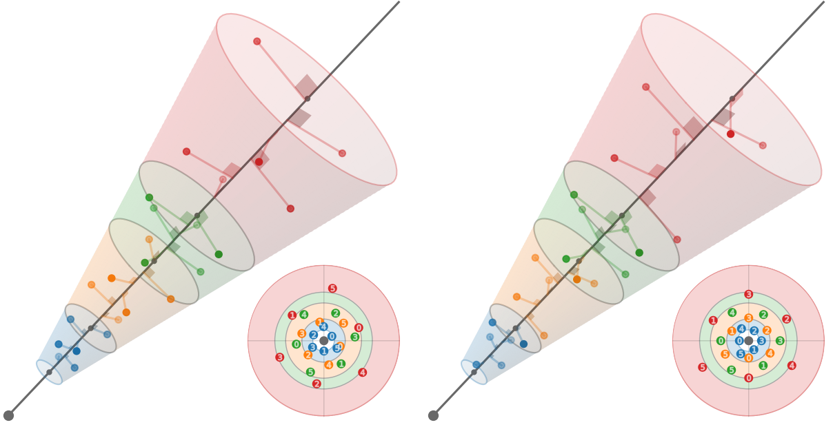
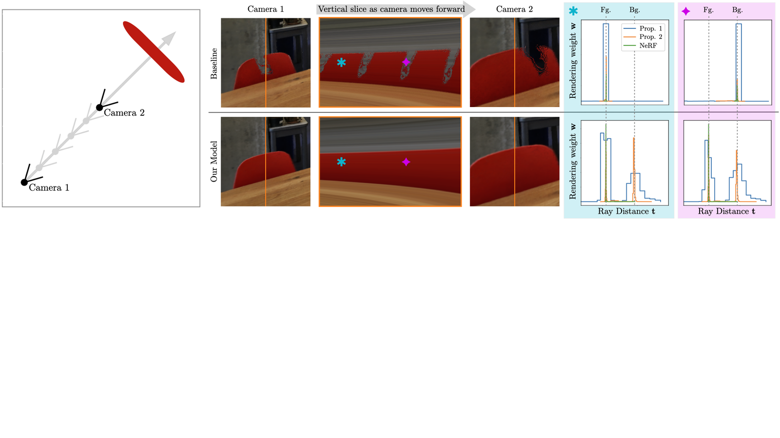
The paper's Figure 2 compares five ways to query a one-dimensional grid: at the Gaussian's mean, by the true convolution, with downweighting alone, with supersampling alone, and with both. That is the experiment I rebuilt below, with numbers.
One iteration, as the code runs it
The default config trains with 65,536 rays per iteration for 25,000 iterations, with 64, 64 and 32 samples per ray for the two proposal levels and the final level (read, zipnerf_garden.yaml). That is 10,485,760 intervals and 62,914,560 multisample points per iteration (computed). Each of the three sampling levels has its own hash grid, and the shapes below are the config's:
| Grid | Levels | Features per level | Resolutions | Table entries | Parameters | Output features |
|---|---|---|---|---|---|---|
| Proposal 0 | 6 | 1 | 16 to 512 | 2^21 from 128³ up | 6.6 M | 12 |
| Proposal 1 | 8 | 1 | 16 to 2,048 | 2^21 from 128³ up | 10.8 M | 16 |
| NeRF | 10 | 4 | 16 to 8,192 | 2^21 from 128³ up | 59.9 M | 50 |
All of this is computed from Model.py: the levels double in resolution, a level is stored densely until size³ exceeds 2^21 entries (128³ is exactly that, so it is dense), and above that it is hashed. The tables hold 77,291,520 parameters, 309 MB in fp32. The MLPs add 229,606: the two proposal networks are 897 and 1,153 parameters, and the NeRF network, with its 64-wide density layers, 256-wide bottleneck and three 256-wide view layers, is 227,556. The feature buffers the forward pass keeps for the backward add up to 1,107 MB at the default batch, more than half of it the NeRF level's fp16 features and inputs. The README says training needs about 10 GB. From the shapes I can account for about 6 GB: those 1.1 GB, about 3.2 GB for the NeRF MLP's three 256-wide fp16 activations over 2,097,152 intervals, 1.2 GB for the parameters, gradients and Adam moments, and the pixels of the training views (computed, so a lower bound). The rest I cannot place without running it.
The trainer (Trainer.training_iteration) calls generate_rays, then render_rays_training, then compute_gradients, then the optimizer. There is no loss.backward(). The loss kernel computes the losses and their gradients in the same pass, and the backward kernels consume those gradients directly.
The featurizer is where the time is
The forward featurizer is a runtime-compiled kernel with one thread per interval (featurize_forward.cu and featurize_common.cuh; read). Here is what one thread does.
Frustum moments. From the interval's two endpoints it computes the mean and half-width, then the constants ratio = h / (h² + 3 s²), base = t1² + 2 s² and a square root, the closed forms of the conical frustum's mean and covariance.
Six points. For j from 0 to 5 the point sits at an axial distance t0 + ratio · (base + (3/√7)(0.4 j − 1) · root) and at radius √0.5 · r · cz from the ray, at an angle of (π/3) × (0, 2, 4, 3, 5, 1)[j], reversed when the interval is flipped and plus a rotation. In training the flip and rotation are random, hashed from the iteration's seed; at inference they alternate with a fixed π/6 rotation, which is the paper's Figure 3.
Contraction. A point outside the unit sphere is mapped by p · (2‖p‖ − 1) / ‖p‖² into a ball of radius 2, which is Mip-NeRF 360's contraction. The point's footprint scale is multiplied by (2‖p‖ − 1)^(2/3) / ‖p‖². I checked the algebra: that is the cube root of the contraction's Jacobian determinant, an isotropic stand-in for what is really an anisotropic stretch (computed from the formula; the code does not say so). The result is mapped into the unit cube by dividing by 4.
Downweight. For every level the weight is approx_erf(1 / (√8 · scale · size)), with approx_erf(x) = sign(x) · √(1 − exp(−4x²/π)). That is the paper's erf with a closed-form approximation, and scale · size is the footprint radius in cells.
Corners. The six points land in cells. Points in the same cell share their eight corners, and their weights are merged before any lookup. A level is read through a dense index up to 128³ and through the hash (x ⊕ y · 19349663 ⊕ z · 83492791) mod entries above. Each corner's weight is its trilinear weight times the downweight, and the accumulated features are scaled by 10 / 6: the official code's feature preconditioning of 10, divided by the six multisamples, so the six points are averaged in the same step. The kernel also writes one extra feature per level, the sum of (2w − 1) over the six points times a per-level magnitude that the optimizer keeps up to date, so the network can see how much of the level survived the downweight.
The network. For a proposal level the 12 or 16 features go through a 64-wide ReLU layer and a linear layer to one raw density. The weights were copied into shared memory at the top of the kernel, so the network costs shared-memory reads, not global ones.
A table row is 4 bytes for the one-feature grids and 16 bytes for the four-feature NeRF grid, read with a single vector load per corner. A comment in the kernel says it is "bound by L2 requests". At inference, rays are processed in Morton order and a warp takes the same interval of 32 neighbouring rays, so its lookups mostly land on the same cache lines. In training the pixels are random, so that coherence is not available, and the kernel is called without the interleave.
How many rows does an interval read?
Merging same-cell points is an optimization about reads, so I measured it. I ported the repo's multisample geometry to numpy and ran it on 3,000 synthetic rays with 64 intervals each (a pinhole camera of 70° field of view and 1,297 pixels, cameras one to two units from the origin; the pixel radius works out to 6.2 × 10⁻⁴). For each level I counted the distinct cells the six points fall in (toy).
At the coarsest level, 77% of intervals have all six points in one cell, so an interval reads 10 rows on average instead of 48. At 512³ it is 37 rows, and by 8,192³ the six points are in different cells almost every time and nothing merges. Summed over a grid's levels: 124.8 rows per interval for the 6-level grid, 213.1 for the 8-level grid and 308.8 for the 10-level grid, against 288, 384 and 480 without merging, which is 57%, 45% and 36% fewer (toy). Across all three grids it is about 2.07 billion row reads per iteration at the default batch, forward only (toy, on uniform intervals; trained proposal levels concentrate samples where density is, which shifts these numbers in a direction I did not test).
What the downweight does
The numbers above count reads. The downweight changes what is read. To see its effect I built the paper's Figure 2 as a measurement. One hash-grid level, filled with independent noise (which is what a fine level looks like before training gives it structure), is read in three ways for intervals of every footprint size, against the Gaussian-weighted average of the same field over the frustum, estimated by Monte Carlo (toy):
- A a single lookup at the interval's centre, as Instant-NGP does;
- B the mean of the six multisample lookups;
- C the six lookups, each scaled by the code's erf weight, then averaged.
Results, averaged over footprint bins (RMS error against the true footprint average; the field itself has RMS 0.54):
| Footprint radius, in cells (levels up to 256³) | A | B | C | Weight |
|---|---|---|---|---|
| under 0.1 | 0.24 | 0.06 | 0.06 | 1.00 |
| 0.5 to 2 | 0.50 | 0.19 | 0.10 | 0.42 |
| 2 to 6 | 0.53 | 0.22 | 0.05 | 0.13 |
| over 6 | 0.55 | 0.24 | 0.03 | 0.04 |
Once the footprint covers a few cells, A is as wrong as it can be, an error as large as the field. B settles at about 0.22, the floor for averaging six independent draws in different cells: 0.54 / √6. Only C keeps falling, because its weights fall toward zero and the true footprint average of noise does too. At footprints over two cells, C's error is 10 to 18 times smaller than A's and 4 to 8 times smaller than B's. That is the whole argument for the weight, and it is the paper's Figure 2 as a table.
The toy also shows something the paper's one-dimensional figure cannot. The weight depends only on the radial footprint, scale, and not on how long the interval is along the ray. For the finest levels (1,024³ and up) with small radii, an interval can span dozens of cells or more along the ray, the true average is small, and C's weight is still 1, so C stays at B's error of about 0.2. In a trained model the fine levels hold structure and not noise, so this is a worst case and not a finding about the repository's quality. It is a limit of a weight that sees only the radial footprint; whether it matters for rendered quality depends on how trained fine levels behave, which this toy does not test.
Why the compiler is part of the design
The featurizer is not compiled when the extension is built. It is compiled when the first training iteration runs (Featurizer::kernel in featurizer.cu; read). The host code writes a preamble of #defines for the number of levels, features per level and MLP width, plus four functions, level_size, level_entries, level_offset and level_hashed, each a switch over the level index. Inside the kernel every level loop is unrolled, so those switches fold to constants: each level's resolution, its table offset and whether it is hashed are literals in the machine code. The kernel source is then compiled with NVRTC, for the device's own architecture when the toolkit supports it and as PTX otherwise, with --use_fast_math, and the binary is cached on disk under a key that hashes the full source and the compiler options. The kernel files are inlined and not included, so editing any file changes the key. The README consequently notes that the CUDA backend "cannot be used as a standalone PyTorch extension".
The post credits tiny-cuda-nn's JIT fusion as its motivation. That library describes the technique in its README (v2.0 and later): it converts a model to a CUDA device function and compiles it with runtime compilation, reports 1.5x to 2.5x for automatic fusion, and says Instant-NGP gets 5x "by fusing the entire NeRF ray marcher into a single kernel" (reported; I read the README at commit 3daa6e5, dated 17 August 2026). The repository does not use tiny-cuda-nn. It has its own NVRTC wrapper, 127 lines in runtime/src/rtc_kernel.cu, and the grid and MLP are its own code. It is the same idea with the library removed.
No autograd: recompute, scatter, reduce
The backward is where fusion usually dies, because a generic framework stores every intermediate for the gradient. This code does something different (read).
- Recompute. The backward kernels do not read stored corner rows or weights.
scatter_feature_gradientsrecomputes the multisample positions and the corner weights from the ray and the interval, the same arithmetic as the forward, and adds into the grid gradient. The random numbers are regenerated from the seed. - Atomics. The grid gradient is accumulated with atomic adds, and for the four-feature NeRF grid on sm_90 and newer with a single vector instruction,
red.global.add.v4.f32. - Proposal levels.
featurize_backward_mlpreads back the stored fp32 features, recomputes the 64-wide layer, scatters the input gradient into the grid, and reduces the MLP's parameter gradients across the block in shared memory so there is one atomic add per parameter per block. - Losses.
train_final_kernelcomposites the final level, computes the Charbonnier colour loss (padding 0.001), the distortion loss (weight 0.01, power −0.25, premultiplier 10,000), and both interlevel losses (weight 0.01, blurs 0.03 and 0.003) against the blurred final weights, and writes every gradient. One thread per ray, with warp reductions for the logged sums. - The NeRF MLP. Six fp16 cuBLASLt GEMMs with fused bias and ReLU epilogues forward and dReLU backward. Gradients carry a static loss scale of 1,024. The 256-wide bottleneck only feeds linear maps, so it is folded into two weight matrices.
- The optimizer. One launch over all buffers: unscale,
nan_to_num, the Adam update, the grid regulariser (weight 0.1) and the per-level scale magnitudes, then zero the gradients.
I did not check the gradients numerically; they are analytic and the repository has no test that does. The README's PSNR is the only evidence that they are right.
What fusion saves
All of the above exists to avoid writing intermediates. To put a size on it, I counted what the featurize-and-MLP stage writes to global memory per interval (read for the fused side, from the kernels' output pointers; assumed for the other, below).
- Fused, training: 52 bytes for the first proposal level (the raw density, 4 bytes, plus 12 fp32 features kept for the backward), 68 for the second, 176 for the NeRF level (112 bytes of fp16 features plus 64 bytes of direction and bias columns).
- Fused, inference: 4 bytes for each proposal level, because the feature pointers are null, and 176 for the NeRF level.
- Unfused, assumed: a straightforward tensor-by-tensor version that materialises the six positions and scales, the corner indices (int64), corner weights, gathered features, one feature vector per level, and for proposals the MLP's 64 pre-activations and 64 ReLU outputs. That comes to 5,268, 6,820 and 13,736 bytes per interval.
At the default batch the unfused version writes 79.5 GB per iteration and the fused one 0.87 GB (computed). If each of those bytes is written once and read back once, 79.5 GB each way takes about 88 ms at 1,800 GB/s, against under 1 ms fused. That is the forward intermediates alone, with no backward, no table reads and no cache reuse.
The README's whole iteration is 85.9 ms (35:47 over 25,000 iterations), forward, backward and optimizer, which is 122 million intervals per second through the full pipeline (computed from the README). So a tensor-by-tensor implementation of this pipeline could not come near that time on a card with memory bandwidth near the 1,800 GB/s I used (the 5090's published peak is of that order; I did not measure it). That is a statement about what fusion has to be doing, and it is reasoned. The unfused column is my assumption and not the official code, which runs under XLA and fuses some elementwise work itself. I cannot say how much of the official implementation's gap this accounts for, and I did not profile any stage. Treat the 88 ms as an upper bound on the effect for a naive baseline.
The same effect on a CPU
A GPU is not required to see the principle. I benchmarked a chain of eight elementwise operations over 16.8 million floats on one thread of a shared Xeon (toy; min of seven runs; the machine was busy, so read the ratios).
Run one pass per operation, the chain takes 95 ms in place and 218 ms when each step allocates its result. The same chain run in cache-sized chunks takes 44 ms at best, and torch.compile fuses it into one loop at 63 ms after a 51-second compile. The gain is real and conditional: chunks that are too small lose to call overhead, chunks the size of the array lose the cache, and the optimum sits between. The unfused chain moves 72 bytes per value in the ideal accounting, the fused one 8. This is the memory-bound effect at CPU scale; it says nothing about the 5090.
The same trade appears at LLM scale in the Kimi K3 decode path on GB300, which fuses the attention projections, the mixture of experts and the all-reduces into 13 kernels a layer instead of 23: when a step's arithmetic is cheap, the cost is the memory traffic around it, and the cure is fewer trips. For the other main route to novel-view synthesis, Gaussian splatting, the trade is different: it spends memory on explicit primitives instead of compute on a network.
The benchmark claim, examined
The README's results, for the garden scene of the Mip-NeRF 360 dataset (the images_4 JPEGs, every eighth image held out), default config:
| PSNR | SSIM | |
|---|---|---|
| Zip-NeRF paper | 28.20 | 0.860 |
| Official code release | 28.22 | 0.863 |
| This implementation | 28.22 | 0.860 |
Training takes 35:47 and about 10 GB of VRAM; rendering a 1,297 x 840 view takes about 300 ms on an RTX 5090. The official implementation "takes about 5 hours to train this scene and renders at 0.1-0.2 FPS on an RTX 4090" (reported, all of it). The README says "we have only run limited tests".
Three things stand out when I check the ratios against these numbers (computed).
- Training. Five hours over 35:47 is 8.4x, not 6-7x. The README does not say which GPU ran the official code for those five hours, so I cannot tell whether the headline reflects an adjustment I cannot see or a different measurement.
- Rendering. 300 ms is 3.3 FPS. Against 0.1 to 0.2 FPS that is 17x to 33x, not 10x, and the two numbers come from different cards, a 5090 and a 4090.
- Quality. PSNR matches the official code at 28.22. SSIM is 0.860 against 0.863, a gap of 0.003 on one scene, one seed and one held-out split. That is close; it is also one data point.
The post's "300 ms per megapixel" is consistent with the README: 300 ms for 1.09 megapixels is 275 ms per megapixel.
None of this says the speedup is not real. A fused, hand-written pipeline with a sound memory argument should be many times faster than JAX on a general-purpose compiler. It says that the headline ratios are not derived from the numbers printed beside them, that hardware is mixed, and that nothing is repeated. The claim I can support from the source is the structural one: this pipeline avoids almost all the intermediate traffic a naive one would have.
"Written with Opus"
The post says it was written with Opus. The repository says nothing about it. I searched every file in the repository, the CUDA sources included, and both commit messages for "Opus", "Claude", "Anthropic", "assistant", "Copilot", "ChatGPT" and "generated by", and found nothing. The git history is two commits by one author. So the claim rests on the post alone. What the repository does show is what stands in for verification: a results table, a note that testing was limited, and no tests. The kernels are 2,815 lines of non-trivial CUDA and C++ with analytic gradients, and the evidence that they are right is a PSNR on one scene. That is a reasonable thing for a one-day-old release and a thing to weigh before building on it. I make no claim about the role of any model, because the repository gives me no basis for one.
What I did not run
- Every line. The optimizer kernel, the ray generation and the compositing helpers I read for structure and comments, not line by line, and I did not read the cuBLASLt algorithm-selection code beyond its comments.
- Anything on a GPU. No kernel was run, compiled or timed. I could not run downloaded code here, and the machine has no CUDA device.
- The official code. I did not run the JAX implementation, so every comparison to it is the README's.
- The gradients. No numerical check against the official code or finite differences.
- Real sample distributions. The row counts use uniform intervals on synthetic rays, and the downweight toy uses noise features.
What would settle it: run the config on a 5090, record the 35:47, profile with Nsight Compute (the build has a ENABLE_NVCC_LINEINFO switch for exactly that) to see which kernel is L2-bound and how much the featurizers cost against the GEMMs, run the official code on the same card, and repeat on a second scene with a few seeds. If those agree with the README, the speedup is real. If the training ratio comes out at 8x on a matched card, the headline was conservative.
Sources
- Repository: fhahlbohm/fused-zipnerf, read at commit
b240dad(31 October 2026). - Paper: Barron, Mildenhall, Verbin, Srinivasan and Hedman, Zip-NeRF: Anti-Aliased Grid-Based Neural Radiance Fields, ICCV 2023; figures 3 and 4 and the description of Figure 2 are from the paper's HTML version.
- tiny-cuda-nn, README section on JIT fusion, commit
3daa6e5. - The post: @fhahlbohm on X, 30 October 2026.
- My scripts and results (layout counts, the multisample geometry port, the footprint toy and the fusion benchmark) are in
public/articles/fused-zipnerf/code/.