2026-08-03 · 14 min · generative-models · diffusion · training-methods · robotics · explainer
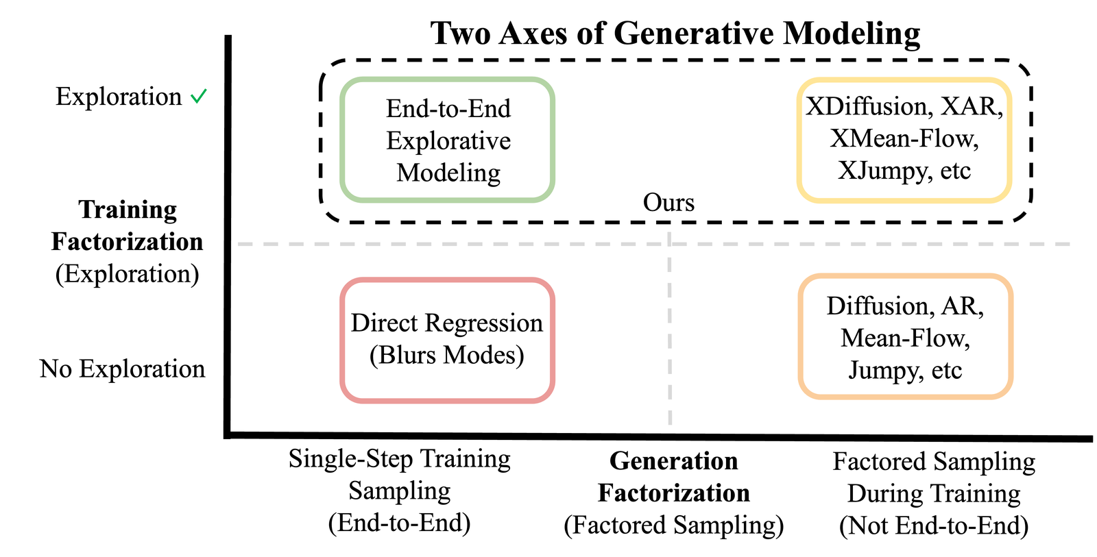
Every generative model has to solve the same problem: a prompt like "generate a dog" has billions of valid answers, not one. Diffusion handles that by denoising in dozens of steps; autoregression handles it by predicting one token at a time. Both are the same trick wearing different clothes — break generation into enough small steps that no single prediction has to average across the billions of valid dogs. Explorative Modeling (Gladstone, Ji, and Du — UIUC and Harvard) asks a different question: what if you left generation alone and factored the training loop instead? Generate candidate outputs per example, score them all against the target, and only backpropagate through the winner. They call this exploration, argue it is a third axis for scaling generative models — next to parameters and data — and show it can substitute for step-factored generation entirely, which is what lets them train models that generate in a single forward pass and still match diffusion.
Why generation gets factored in the first place
Squared-error regression is maximum likelihood — under a fixed-variance Gaussian. That sounds like a technicality, but it has teeth: the maximum-likelihood-optimal output under a multimodal target is the mean of every valid answer, and the mean of "every plausible dog photo" is not a photo of a dog. It is a brown blur. Same failure in language: force a next-token model to average over "the cat sat on the _____" and you get a smear of probability mass spread across every plausible word, not a committed answer. The paper gives this capacity a name, generative expressivity: the number of distinct modes a training objective's loss minimizer is allowed to capture. A direct regressor has expressivity — one output, always the average — and no amount of extra parameters or data raises it, because expressivity is a property of the objective, not the model.
That is the reason diffusion and autoregression look the way they do. Autoregression conditions each token on everything already generated, so by the time it predicts token , most of the multimodality is already resolved by the tokens before it — each individual prediction is closer to unimodal. Diffusion does the analogous thing over noise levels: each denoising step only has to move a slightly noisy sample a little cleaner, not solve the whole distribution at once. Factoring generation is a device for keeping generative expressivity high, one small step at a time. It is also why training and inference stop matching: a diffusion model trained on isolated denoising steps gets unrolled over hundreds of them at test time, and even single-step distillations still anchor their training targets to the multi-step trajectory. Sampling and training are never the same procedure, so exposure bias never fully goes away.
Forward XM: buying expressivity with candidates, not steps
If factoring generation is one way to raise expressivity, exploring more candidates is another. Fix a data target , draw generations from the model, and train only on the closest one:
This is the entire mechanism — no new architecture, no new loss family, just a for loop around
generation and a min before .backward(). Explore candidates with a plain regressor and its
expressivity rises to at least : with enough candidates, one of them lands near enough to any given
mode that the model can commit to it instead of averaging.
Every candidate is scored against the same target; only the nearest one back-propagates, the rest are dead ends for this step. Pulling K up can only tighten the best-of-K error, never loosen it — but each extra candidate is a full generation, so the win is bought with training-time compute, once, not with a longer inference pipeline you pay for on every sample.
Play with above and the mechanics of equation (1) are exactly what's on screen: every candidate is scored against the same target, the closest one gets the gradient, and the rest are discarded for this step. Pulling up can only tighten the best-of- error — never loosen it, since you are taking a minimum over a strictly larger set — but each extra candidate is a full extra generation, so the compute for a training step scales linearly with . That is the whole cost of exploration, and it is paid once, during training.
The same de-blurring shows up in the model's actual outputs, not just the training loss:
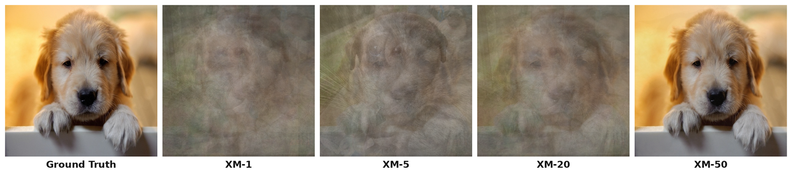
XM-1 is not a badly-trained model — it is the theoretical best a direct regressor can do, the blurred mean equation (1) predicts. XM-50 is the same architecture, same data, same loss, with one difference: 50 candidates scored per step instead of one.
Forward and Reverse XM, and what they actually optimize
Forward XM (fix the data, explore the model's generations) is one direction. Reverse XM flips it: fix one generated sample and explore over data targets , training toward whichever is closest:
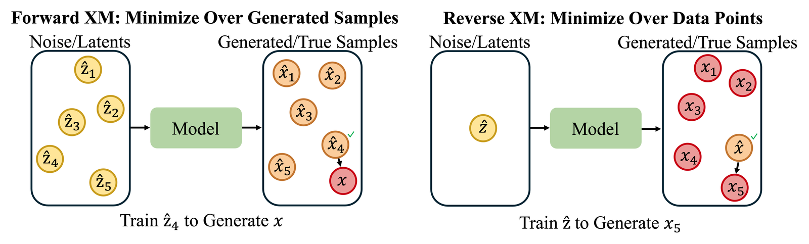
These are not cosmetically different. The paper works out what each one minimizes in the limit. Write for the model's output distribution blurred by the reconstruction kernel (Gaussian, for squared error) and for the data blurred the same way. Then, in their smooth relaxations:
Forward XM's entropy term, , belongs to the data — a constant the model can't touch — so Forward XM is just maximum likelihood over its -candidate mixture, for every . Mass-covering, never collapsing, but the recall comes at the price of running full generations per step, so it struggles to scale to very high-multimodality targets. Reverse XM's entropy term, , belongs to the model — something it can shrink by narrowing its own spread — so Reverse XM drifts toward collapse on its own and needs an explicit entropy bonus to stay at the true reverse-KL optimum instead. The paper is candid that Reverse XM's fix is "largely left for future work"; Forward XM is what every downstream result in the paper actually runs.
Substitutable, not just additive
Here is the move that turns this from "a training trick" into "a scaling axis." Factoring generation exists only to supply expressivity. Exploration supplies the same quantity a different way. If that's right, the two should be interchangeable — you should be able to trade generation steps for exploration and land in the same place. The paper tests this directly with Jumpy models, a family that interpolates between direct regression (one jump) and full continuous-time flow (infinite jumps) by varying the number of steps. Take two Jumpy models, one with fewer jumps and one with more, and add exploration to both: the model with fewer jumps — the more end-to-end one — gains more from exploration than the one that already had step-factorization doing the work. That is the substitution effect, measured rather than asserted: the less a model already leans on factored generation, the more it has to gain from factoring training instead.
Push that trade all the way and you get XM's other headline: a model that samples exactly the way it trained, in one forward pass, with no separate multi-step inference procedure to keep in sync. The paper calls a model "end-to-end" when it never faces inputs at inference it wasn't trained on — no denoising schedule to unroll, no exposure bias from a mismatched sampling procedure. This is the same argument that ended hand-designed feature pipelines after AlexNet, aimed now at the one corner of deep learning that never fully got the memo: diffusion language models and autoregressive decoding both still train on one procedure and sample with another; exploration is what lets a model close that gap without giving up quality.
The trade is exactly compute, moved to a different place in the pipeline:
The explorative line is flat because its training paid a one-time premium (8× extra generations per step, spent once) so inference could drop to a single forward pass. The step-factored line keeps climbing because every one of its 50 samples pays the full step count again. Drag to 100 or 256 steps — the actual NFE gaps the paper measures on Diffusion Policy and Diffuser — and the ratio lands right around what it reports, even though these particular unit costs are illustrative.
MrFlow and Set Diffusion both attack the inference side of this same step-factorization: reshuffle where a fixed step budget gets spent, or change which tokens get decoded together, but the sample is still built from many forward passes. Explorative Modeling is a different lever entirely — it doesn't make the multi-step generator cheaper, it removes the requirement to be multi-step in the first place, by paying for expressivity up front instead of on every draw.
Results: three modalities, two robot benchmarks
Image generation. Added to RAE, a near-state-of-the-art ImageNet latent-diffusion recipe, exploration (XRAE, using XM-2) reaches a near-SOTA 1.43 FID without classifier-free guidance:
| Method | FID (no CFG) ↓ |
|---|---|
| DiT | 9.62 |
| SiT | 8.61 |
| VA-VAE | 2.17 |
| REPA-E | 1.70 |
| Latent Diffusion + RAE | 1.55 |
| XRAE (RAE + XM-2) | 1.43 |
That 47% parameter-efficiency figure is unrelated to the next number, which happens to share a digit: RAE itself converges 47x faster than SiT (a separate, prior result the paper is building on), and stacking XRAE's 6.2x sample efficiency on top of that puts the whole recipe at roughly 300x faster to converge than plain SiT — the paper's arithmetic, not an independent measurement. One negative result worth keeping: minibatch optimal-transport coupling, an alternative de-blurring trick, made FID worse (46.3 → 54.5 at the Small scale) — exploration wins here specifically, not "adding any anti-blur trick" generically.
Scale doesn't dilute the gain — it grows it. Going from XM-5 to no exploration, the improvement climbs from 13% to 23% as model size scales up, and from 7% to 36% as data scales up. That is the opposite of what you'd expect from a scaling axis that's about to run out of room — the paper's reading is that generative expressivity becomes a larger bottleneck as the other two axes get pushed harder, because parameters and data stop being the limiting factor first.
Video (Something-Something V2). FID/FVD improve monotonically with more explored modes. The more interesting number is generalization, not fit: best achievable FVD is 30.0 with exploration versus 37.5 without — less overfitting on a fixed dataset, which the paper frames as a compute-generalization tradeoff: extra training compute spent on exploration buys generalization the way more data usually does.
Robot policies (Behavior Cloning, Robomimic). This is where "single forward pass, matches diffusion" gets tested against a real baseline:
Explorative Policy matches Diffusion Policy on Lift and Can (both 100%), and beats it on Square (96% vs. 94%), Transport (74% vs. 72%), and ties on Tool Hang (86%) — at 1 forward pass instead of 100.
Goal-conditioned world models (Maze2D), vs. Diffuser:
Average score edges up too (130.0 vs. 127.2), at 16-256x fewer denoising steps depending on the maze size (4 vs. 64 on U-Maze, 1 vs. 256 on Medium). This pairing — matching or slightly beating a strong multi-step baseline, at two orders of magnitude less inference compute per sample — is the article's headline for a reason: it is the plainest demonstration that the compute the paper claims you save at inference is compute it actually spent, once, at training.
What I make of it
- The conceptual reframe is the real contribution. "Factor the training loop instead of the generation loop" is a genuinely different axis, not a repackaging of an existing trick — best-of- training has appeared before, but treating it as substitutable for diffusion/AR step-factorization, and confirming that substitution empirically with the Jumpy-model ablation, is new.
- "Third scaling axis" is the authors' framing, argued from one paper's worth of experiments — real equations, a real KL derivation, and empirical scaling curves that trend the right way, but not yet a claim anyone outside this group has stress-tested. Treat it as a strong hypothesis with supporting evidence, not an established fact.
- The evaluation is real but narrow at the edges that matter most. The robotics results — the ones carrying the "matches diffusion at 100-256x less inference compute" headline — are Robomimic proficient-human/state-observation behavior cloning and Maze2D planning: small, well-studied benchmarks, and the paper says outright the control experiments got "barely any tuning." That's stated as a limitation working in XM's favor (untuned and already competitive), but it also means these are not yet frontier-scale robot-learning results, and there's no evidence here about vision-based control, long-horizon manipulation, or real hardware. Gains on autoregressive language models are the weakest reported of any modality — the paper's own explanation is that next-token prediction is already close to unimodal, so there's less blur left for exploration to fix.
- Code is Apache-2.0 and real, which counts in its favor —
--xm_best_of_k Kis a genuine flag in a runnable repo, not a promise. But as of this writing the repository explicitly marks the code behind the headline results as not yet released: the RAE image-generation runs use a separate codebase "to be released separately," and masked-diffusion-language-model and control-task (robot policy / world model) code are both marked "coming soon." What's public today is the general XM training scaffolding, not a drop-in reproduction of the paper's own numbers. - No third-party replication yet — the paper is a July 2026 preprint. The authors are transparent about a related limit: Diffusion Policy's numbers had to be reproduced under their own setup because they used a newer Robomimic version than the original paper, so the baseline is a good-faith re-run, not a quoted number — a small but real point of honesty worth crediting.
The clean way to hold all of this: exploration is a training-time payment for a capability generation factorization normally buys at inference-time, over and over. That's a real trade, mechanically well argued, and it works on real benchmarks. Whether it holds at frontier model scale, on harder control tasks, or once other labs have run the numbers, is still open.
Built on Explorative Modeling: Unlocking a Third Pretraining Axis and End-to-End Generation (Gladstone, Ji & Du — UIUC and Harvard, 2026). Code: github.com/alexiglad/XM (Apache-2.0). Figures 1-3 are reproduced from the paper; all numbers are from its Tables 1-3 and Sections 4.1-4.2.