2026-08-23 · 8 min · robotics · world-models · vla · multimodal
Why read this
Solidtop 85%How one shared latent space makes Flex-pi's inputs and outputs runtime flags, and why 11 of 20 eight-stage repairs is 93% per stage against 69%.
- Runs on a consumer GPU
- A new technique
- Explained from first principles
Robotics & embodiedMITResearch model
How this was scored
- Is it new?
- 2 of 3: A real new idea, method or capability
- Can I trust it?
- 1 of 3: Spot-checks a few numbers
- Can I run it?
- 2 of 3: Open code or weights with real limits
- Will I understand it?
- 2 of 3: Mechanism from first principles with figures
- Can I act on it?
- 1 of 3: General advice
- Will it last?
- 1 of 3: Relevant for months
- Does it affect many?
- 1 of 3: A specialist community
- Only here?
- 1 of 3: Some original analysis
Score 48 of 100, ranked 482 of 577 rated articles. Each question is answered 0–3 by hand, and a 3 is rare. How articles are scored
World-action models predict the future so they can act better. In practice they predict RGB latents trained for pixel reconstruction, which is a strange choice for manipulation: nothing in that objective supplies the 3D geometry or object semantics that picking things up actually depends on.
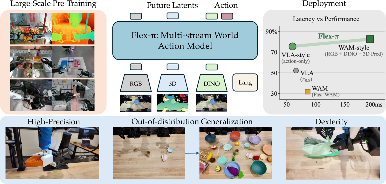
Flex-π predicts all three. RGB appearance, 3D pointmap geometry and object-centric DINO semantics get denoised jointly with the action in one shared latent space — and because they share that space, dropping one at inference is a masking operation rather than a different model. What it reads and what it generates become runtime arguments, so a single checkpoint covers 56 deployable configurations from VLA-speed action-only inference to full joint generation.
| Paper | arXiv:2608.10860 · Yan, Liu, Fan, Cai, Liao, Zhang†, Fox† · UW + AI2 |
| Code | geyan21/flex-pi, MIT · project page |
| Model | 6B parameters · frozen Wan-2.2 VAE (RGB and pointmap) + frozen DINOv3 |
| Flexibility | 56 input/output stream combinations from one set of weights |
| Latency | 60 ms action-only, 193 ms full joint, on an RTX 5090 |
| Real robot | bimanual YAM workcell · 83.0% task completion in distribution, 76.1% out |
| Against π₀.₅ | 52.1% → 43.2%. Flex-π drops 2.5 points where π₀.₅ drops 37.5% of its performance |
Three streams, one latent space
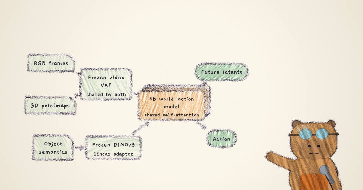
The move that makes the rest work is smaller than it sounds. RGB frames and 3D pointmaps go through the same frozen video-generation VAE — not a geometry encoder alongside a visual one, the same weights — because a VAE trained only on RGB already encodes depth well enough to reconstruct a pointmap at 31.1 dB PSNR and 4.9 cm z-RMSE. DINO semantics come from a separate frozen encoder, projected in by a linear adapter. Proprioception and the language instruction condition every stream.
Crucially the model predicts future observations as latents from those pre-trained encoders, not as pixels. Each encoder's priors carry over, the joint representation is stronger, and inference is faster because nothing has to be decoded — actions are generated jointly with the latents under shared self-attention, so the policy reads its own predicted future without ever rendering it.
The flexibility comes from per-stream dropout during training, plus something the authors call cross-modality forcing: the model is trained to predict each modality's future even when that stream is missing from the input. This alone raises RoboTwin success by 47% relative.
That is worth separating from the robustness story it enables. Requiring each modality to be predictable from the others is what stops the shared backbone from quietly splitting into three weakly-coupled channels — it pushes toward a representation where appearance, geometry and semantics are mutually predictive. Surviving a missing sensor is the by-product, not the goal, and it is why the 56 configurations are deployable without fine-tuning any of them.
What it buys on a real robot
The in-distribution numbers are good and unremarkable: 83.0% against 58.0% for the strongest baseline. The out-of-distribution column is where the design shows.
Clutter the workspace with novel distractors and swap in object types the policy never handled, and π₀.₅ loses 37.5% of its performance while Flex-π's joint mode loses 2.5%. ManiFlow, which has explicit 3D inputs of its own, loses 27.5%. On the unseen soft bag — fabric that shifts under every grasp, so the zip never stays put — the comparison is 63.3% against 6.9%.
And the half-data condition is the number I would put in front of anyone deciding what to fund. Flex-π trained on half the demonstrations, running action-only, scores 80.0% on Put Plate against π₀.₅'s 42.5% on the full set. Demonstration collection is the binding constraint in real robot learning; a method that extracts more per episode is worth more than one that is faster.
Eight stages, in order
The hardest task in the suite is a robot repairing its own gripper: eight stages that must complete in sequence, split between two moving arms, with an electric screwdriver and a sub-millimetre insertion near the end.
Flex-π in full joint mode finishes all eight stages in 11 of 20 rollouts. The best baseline manages it once.
An eleven-fold gap in end-to-end success sounds like a difference in kind. Take the eighth root and it is about 93% per-stage reliability against about 69% — twenty-four points, compounded eight times. That cuts both ways, and I think it is the most useful thing to take from this task: a policy can look competent stage by stage and be useless end to end, and a per-stage improvement small enough to dismiss as noise is worth an order of magnitude wherever the stages are ordered and unskippable.
The recovery behaviour is the other thing the videos show that the table cannot. On the two tightest stages the policy misses, pulls back, re-centres and tries again — which also means the independence assumption above is wrong in a direction that makes the real gap sharper, not milder.
What it costs
The project is unusually direct about its limitations, and both are real.
Joint generation costs about 3× the latency of the action-only path — 193 ms against 60 ms — and the two operating points cannot be had at once. The framing of "compute flexibility" is accurate but it is a choice, not a free lunch: you get VLA latency or WAM accuracy, decided per deployment. What is genuinely new is that the decision moved from training time to runtime.
It is still data-hungry. Flex-π gets more out of each demonstration than the baselines, and the absolute number of demonstrations it needs is still large. The half-data result is a ratio, not an absolute.
I would add a third. The inference-optimization table is training-free and the numbers are good — 447 ms down to 193 for the joint path, 132 down to 60 for action-only — but the fast joint path depends on TensorRT KV-split engines. That is a lot of deployment-specific machinery standing between the checkpoint and the headline latency, and the paper's frontier plot is drawn at the optimized end. Without TensorRT the joint path is 360 ms, which moves the operating point noticeably.
What I would want measured next
Fifty-six configurations, two of them evaluated. The whole architecture exists to make intermediate points deployable, and the paper reports the endpoints. Does predicting geometry without RGB recover most of the joint-mode accuracy at closer to action-only latency? That is the question the design was built to ask, and it is a flag flip away.
Cross-modality forcing is measured on RoboTwin only. A 47% relative gain is the largest single ablation number in the project, and it is reported on the simulator rather than on the real workcell where the out-of-distribution claims live. If it is doing what the authors say — keeping the backbone from splitting into three channels — the real-robot OOD column is exactly where it should show.
Fast-WAM is missing from two of five tasks. It was not run on Self-Repair Gripper or Soft-Bag Zipping, so its averages cover three tasks against everyone else's five. The page says so plainly, which is right, but it means the WAM baseline's average is not comparable to the others' and the "beats every baseline" claim rests on the two it did run.
The idea worth stealing
Strip the robotics and what is left is a claim about representation: if three modalities live in one latent space and are trained to be mutually predictive, then which ones you use becomes a deployment parameter rather than an architecture.
That is not specific to manipulation. Most multimodal systems bolt encoders onto a backbone and fix the set at training time, which is why running them with one sensor missing means retraining or degrading unpredictably. Flex-π's answer — per-stream dropout plus a forcing objective that makes each stream reconstructible from the others — turns the modality set into a mask.
The 56 configurations are the demonstration. The transferable part is that a single frozen video VAE turned out to encode enough geometry to serve as a pointmap encoder too, and nobody had to train anything to find that out.