2026-07-20 · 6 min · pretraining · attention
Why read this
Nichelast 15%Explains differential attention, PolyNorm and Motif's linear data-mix schedule, with the report's code and math scores against 7-8B models.
- Runs on a consumer GPU
- Explained from first principles
LLM architecturePractitioner model
How this was scored
- Is it new?
- 1 of 3: An incremental tweak
- Can I trust it?
- 0 of 3: Restates claims
- Can I run it?
- 2 of 3: Open code or weights with real limits
- Will I understand it?
- 2 of 3: Mechanism from first principles with figures
- Can I act on it?
- 1 of 3: General advice
- Will it last?
- 1 of 3: Relevant for months
- Does it affect many?
- 1 of 3: A specialist community
- Only here?
- 1 of 3: Some original analysis
Score 38 of 100, ranked 539 of 577 rated articles. Each question is answered 0–3 by hand, and a 3 is rare. How articles are scored
Most "small strong model" reports are the same model everyone else ships — a dense pre-norm Transformer with RoPE, GQA, and SwiGLU — trained on better data. Motif Technologies' Motif 2.6B (arXiv 2508.09148) is not that. It makes two architecture bets that mostly live in papers, not products — differential attention and a learned polynomial activation called PolyNorm — and it's the first model I've seen train both at real scale (2.5T tokens). The result is a 2.6B model that goes toe-to-toe with 7–8B models on code and math. Two mechanisms, a data schedule with a plan, and a couple of training tricks make it work.
- architecture
- MotifForCausalLM
- task
- text-generation
- license
- apache-2.0
- safetensors
- 3 shards
- largest file
- 4.97 GB
- files
- 17
- downloads
- 475
- likes
- 88
- languages
- en, ko
repo last modified 2025-08-28
The block
Motif is a 32-layer, hidden-size-2048 dense Transformer — 16 attention heads, no GQA (16 KV heads), a 219,520-token vocabulary, RoPE with θ = 500,000. Standard pre-norm skeleton. What's swapped in are the two coloured boxes: the attention sublayer is Differential Attention, and the feed-forward sublayer's nonlinearity is PolyNorm.
![Motif 2.6B architecture: a pre-norm block with a Differential Attention sublayer that projects Q1, Q2, K1, K2, V and computes [softmax(Q1 K1ᵀ) − λ softmax(Q2 K2ᵀ)]V followed by GroupNorm, and a feed-forward sublayer whose PolyNorm activation combines normalized X, X², and X³.](https://media.thesatyajit.com/ai/articles/motif-2-6b/fig1.png?v=441376f7f51052fc)
These weren't picked by taste. Motif ran controlled ablations at 0.6B, 1.8B, and 4.6B under a fixed 3e20-FLOP budget, testing QK-Norm, Cross-Layer Attention, and Normalized GPT (nGPT) alongside these two — and differential attention plus the polynomial activation are what survived.
Differential attention
Ordinary attention leaks. A softmax over the whole context puts non-trivial mass on tokens that have
nothing to do with the query — the more filler in the window, the more the signal gets diluted.
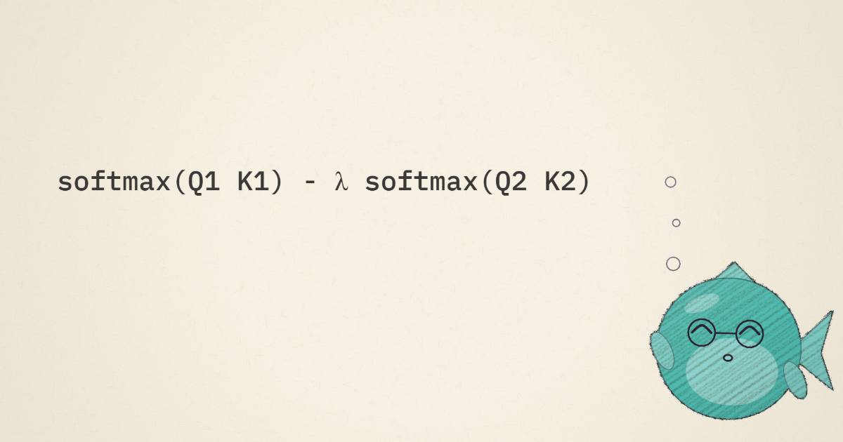
Differential attention (Ye et al.) fixes this by computing two attention maps per head and
returning their difference: attn = [softmax(Q₁K₁ᵀ) − λ·softmax(Q₂K₂ᵀ)]V. The second map is trained
to model the common-mode noise, so subtracting a λ-scaled copy of it cancels the leak. Drag λ:
It's the same move as a differential pair in analog circuits, or noise-cancelling headphones: measure the noise separately, subtract it, keep the signal. Sparser attention shows up downstream as better long-context retrieval, less hallucination, and cleaner in-context learning — and a GroupNorm after the subtraction keeps the (now possibly negative) scores stable.
PolyNorm
The other swap is the activation. Instead of committing the whole network to one fixed curve, PolyNorm
makes the nonlinearity learned: a degree-3 polynomial over normalized powers of the input,
PolyNorm(x) = a₁·n(x) + a₂·n(x²) + a₃·n(x³). Each layer learns its own aᵢ, so it can bend toward
near-linear, saturating, or S-shaped as needed, and pick up higher-order interactions a single
activation can't. Mold it:
The per-power normalization is the load-bearing detail — it's what stops the x³ term from exploding the activation scale, which is exactly why cubic activations don't normally survive contact with a real training run. Motif's is capped at degree 3 on purpose.
A schedule for the data
Here's the training idea I like most. Motif runs a data-mixing scheduler — a schedule for the corpus, conceived like a learning-rate schedule. The 2.5T-token dataset is partitioned into eight domain groups whose sampling ratios move linearly from a start mix to an end mix across training. Drag the training-progress handle:
Early training is broad and web-heavy, teaching general language; the final, best-behaved tokens pour into Korean, code, math, and reasoning — the dense skills the model will actually be graded on. The base corpus is aggregated and filtered from DCLM, TxT360, FineWeb2, and FineMath, plus an in-house Korean corpus (there wasn't a good open one).
Two more training details are worth stealing. The LR follows WSD (warmup-stable-decay): a peak of
5e-4 held flat for the first 2T tokens, then annealed to 25% of peak over the final 0.5T. And
throughout, Motif does checkpoint averaging — every 8B tokens it takes a simple moving average of
the six most recent checkpoints and feeds the averaged weights straight back into the training loop,
a cheap, continuous smoothing that costs nothing at inference. A stage-2 anneal (~500B tokens) then
stretches RoPE from θ = 10,000 to 500,000 (ABF) and extends context 4K → 16K for the long-context
variant in the last 80B tokens.
The finetuning stack
The post-training is where the reasoning gets sharpened. SFT is small — under 15B tokens, ~5M samples — but heavily engineered.
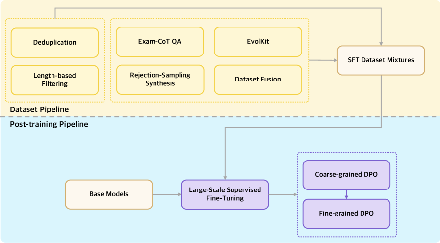
A few of the moves are unusually specific. Exam-CoT QA synthesizes ~5M standardized-exam multiple-choice items with step-by-step rationales. EvolKit (Auto Evol-Instruct, with Qwen3-8B) rewrites existing SFT samples into harder ones. And dataset fusion compresses several samples into one cohesive conversation — they found Qwen3-8B just concatenated the inputs, so they used GPT-4o to actually fuse them, packing more knowledge per token. Rejection sampling against a reward model prunes the weak generations. Then alignment is two-stage DPO — coarse-grained (Tulu 3 preference mixtures) then fine-grained (MagpieLM + LMSys arena data).
Punching above its weight
The scoreboard is the point of all of it. On code and math, a 2.6B model lands where 7–8B models do — and sometimes past them:
On HumanEval it's within a point of Llama 3 8B and more than doubles Mistral 7B; on MATH it clears Mistral 7B by 3×. GSM8K tells the same story — 75.7 (8-shot, maj@8) against Mistral's 52.2. The honest caveat is knowledge: on MMLU the smaller model can't fake breadth.
MMLU rewards parameters you simply don't have at 2.6B, so Motif trails the 7–8B models there while still beating Gemma 2 2B. That's the shape of the whole result: reasoning and code you can train in with the right architecture and data schedule; raw knowledge still scales with size.
The take
Motif 2.6B is a bet that the small-model recipe isn't finished — that there's still room to change the architecture, not just the data. Differential attention buys cleaner attention, PolyNorm buys a learned nonlinearity, the data scheduler front-loads language and back-loads skill, and WSD plus checkpoint averaging smooth the ride. None of it is exotic in isolation; the report's contribution is showing the combination survives 2.5T tokens and lands a 2.6B model in 7–8B territory on the things you can teach. The pieces that "only work in papers" turn out to work in a model — which is the most interesting kind of result.
Source: the Motif 2.6B technical report (Motif Technologies) and its model card. Figures are the paper's; the interactive diagrams are mine. Differential Attention is from Ye et al.; the polynomial-activation idea predates PolyNorm's use here.