2026-09-09 · 23 min · llm · looped-transformers · recurrent-depth · scaling-laws · mixture-of-experts · architecture · explainer
Virtual logic depth, covered on this site last week, made one criticism the loudest: every comparison in that paper — and in the wider looped-transformer literature it sits inside — is parameter-matched, never compute-matched. Loop a block times and you spend roughly the per-token FLOPs of the unlooped model you're being shown beating. Tie the weights and parameters barely move, so "looping buys reasoning for free" survives on one ledger only. That piece named the missing experiment and stopped there, because nobody had run it.
SMELT: Scaling Laws for Compute-Matched MoE Looped Transformers (arXiv 2609.01343, Wang, Zhang, Luo, Wu, Liu, Liu, Huang, Yan, Li — Tsinghua, ByteDance Seed, M-A-P, TokenWave.AI) runs it. Worth being precise about the relationship: this is not a reply. SMELT was posted September 1, 2026, a week before virtual logic depth ran on this site, and its reference list doesn't include that paper — the two are unconnected. What makes them worth reading together is that SMELT's own related-work section states the identical gap, in almost the same words: "most other works above compare looped models against parameter-matched baselines, so the reported gains conflate architectural advantage with the extra FLOPs that repetition spends." Two independent groups looked at the same body of work and flagged the same hole. SMELT is the one that went and filled it.
What "matched" has to mean
Holding one budget fixed is easy; holding three at once is the actual problem. A model comparison can fix:
- Per-token FLOPs — what training and inference actually cost.
- Total parameters — what bounds how much the model can memorize.
- KV cache — what bounds how much context a deployment can serve.
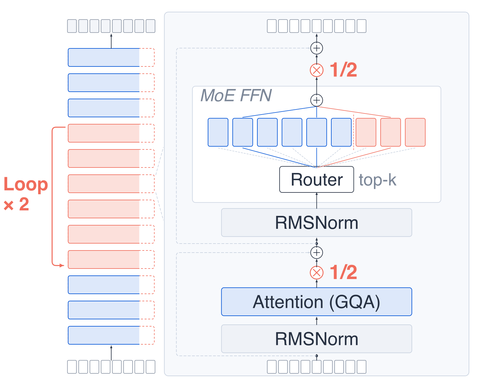
Loop a dense transformer's middle span times without touching anything else and effective depth grows from to for a span of layers. Parameters stay flat — the whole point of tying weights. But FLOPs grow in proportion to , and so, on a naive reading, does the KV cache the extra passes would need. Fix parameters, and the other two float loose. SMELT's fix is to make the model Mixture-of-Experts: MoE decouples total stored parameters from per-token active compute, so a looped model can narrow its hidden width to pay for the extra passes in FLOPs, then buy back the parameters it just gave up by adding experts to the now-larger pool. KV parity comes from a third, separate knob — head size and GQA ratio. Three budgets, three different levers.
Switch to Naive loop and only one bar stays where a parameter-matched paper reports it — params, because tied weights are free by definition. FLOPs and KV cache both drift to 1.5×, uncounted in most of the looped-transformer literature. Switch to SMELT-matched and all three bars snap back near the baseline line — not by refusing to pay for the extra depth, but by narrowing the model elsewhere (width down, expert count up) until the bill comes out even. Effective depth rises 12→18 (×1.5); SMELT states FLOPs “grow in proportion” to effective depth when width is unchanged — we apply that same stated proportionality to KV cache. The paper never runs this uncompensated configuration; this bar is our extrapolation from their Sec. 3.2 relation, not their measurement.
That's the mechanism, made concrete on the one worked example the paper walks through by hand (Sec.
3.2): a 200M-active-parameter MoE backbone, 12 physical layers, looping the middle 6 twice. Left
uncompensated, that's a 1.5× FLOPs tax nobody in the literature is paying. SMELT pays it by shrinking
from 1280 to 1056 and raising the per-layer expert pool from 192 to 288 — landing within the paper's
own reported tolerance (under 4% on every budget; the 200M/S≈95% cell measures +2.9% FLOPs, +0.4%
params, +3.1% KV cache, exact from Appendix A). SMELT does this at three compute-equivalent sparsity levels
(S ≈ 85%, 95%, 97%, defined via Eq. 1 in the paper as the share of parameters a config's FLOPs imply
are inactive relative to a fully-active control) and four model scales.
The literature this sits inside, extended with the papers this site has already covered plus SMELT's own Table 1 (papers not in SMELT's own comparison are marked below; ✓ = matched, ✗ = unmatched or grows with loop count, (✓) = partially matched):
| Work | Arch. | Loop span | FLOPs | Params | KV | Scale tested | Key finding |
|---|---|---|---|---|---|---|---|
| Huginn (2502.05171) | Dense | Mid. 50% | ✗ | ✓ | ✗ | Fixed size (3.5B) | Prelude-recur-coda looping improves reasoning; extra FLOPs uncontrolled |
| Ouro (2510.25741) | Dense | Full (100%) | ✗ | ✓ | ✗ | Fixed size (1.4-2.6B) | Full-stack looping improves reasoning; extra FLOPs uncontrolled |
| Virtual Logic Depth (2506.18233)* | Dense | Full (100%) | ✗ | ✓ | ✗ | Fixed size (50M-200M, one 3B fine-tune) | Reasoning up, knowledge capacity flat, at fixed params; no FLOPs accounting anywhere |
| Schwethelm et al. (2026) | Dense | Mid. (67%→33% as rises) | ✓ | ✗ | ✓ | Iso-depth law (25M-1.6B) | recurrences ≈ unique-block equivalents; looping loses |
| Prairie et al. (2026) | Dense | Mid. 33% | ✗ | ✓ | ✗ | Scaling law at fixed params (100M-1.3B) | Optimal grows with compute; FLOPs and KV grow with too |
| LoopMoE (2606.04438) | MoE | Mid. 33% | ✓ | ✓ | ✗ | Fixed size (3B, 9B) | Wins 8/9 benchmarks at 3B, 9/9 at 9B |
| Nanbeige4.2-3B (2607.22083)* | Dense | Full (100%) | ✗ | ✓ | ✗ | Fixed size (3B, shipped) | Retains ~75% token efficiency at loop ×2; beats 9-12B unlooped models — not FLOPs- or KV-matched against them |
| Full-bandwidth transformer (2608.08888)* | Dense | N/A — vertical feedback, not a layer loop | (✓) | ✓ | ✓ | Fixed size (1B) | Reports its own token-equivalent compute; headline gain still measured against raw-token, not compute-matched, baselines |
| SMELT (ours) | MoE | Mid. 50% | ✓ | ✓ | ✓ | Scaling ladder (0.1B-54B non-embed.) | Wins; 6.8-18.0% training-FLOPs saving on the fitted frontier |
*Rows added for this piece, extending SMELT's Table 1; not in the paper's own comparison. Full source citations follow this article's other coverage: Huginn/Ouro design axes, virtual logic depth, Nanbeige4.2-3B, full-bandwidth transformer.
Read down that column of X marks and the pattern is obvious: almost nobody matches all three, and the ones that match FLOPs (Schwethelm, LoopMoE) don't match params, or vice versa. SMELT is the first block-level looping study to close all three simultaneously across a multi-scale grid rather than one scale.
The recipe, and why each rule survived an ablation
SMELT is not a new mechanism — it's a locked-down set of answers to three design questions, each settled by a controlled sweep at 200M before anything scaled up.
Rule 1 — loop the middle half, not the full stack. Sweeping which contiguous span of a 12-layer backbone loops twice, from 0% (Baseline) to 100% (full-stack, Ouro's regime), validation loss bottoms out near 50% at both sparsity levels tested. The paper reports this as a bare table (Table 3.3); every value in it, plotted:
Hover a point. At both sparsity levels the curve dips near 50% span — loop the middle 6 of 12 layers twice, not all 12 (100%, Ouro’s regime) or none (0%, Baseline). That minimum is why SMELT loops a middle span rather than the full stack: the first and last layers do specialized work that repetition doesn’t improve.
Full-stack looping — what Ouro does, what most of virtual logic depth's Cycle pattern does — is not the
best answer once you control for span. The first and last layers do specialized work that repetition
doesn't improve; looping them anyway is wasted depth. Worth flagging the one place the two metrics disagree:
at S≈95%, DCLM Core (a real downstream accuracy suite) actually peaks at 67% span and dips at
50% — the opposite ranking from validation loss. SMELT picks the span on validation loss, which averages
over billions of tokens and moves smoothly, and treats DCLM as "a consistency check rather than a selection
criterion." That's a defensible call, but it's also the paper being honest that its own two metrics didn't
agree on this particular knob.
Rule 2 — give the looped model a deeper-relative-to-width ratio than the Baseline. With span fixed at 50%, sweeping physical depth under the same three-budget matching finds the Baseline's own optimum at physical depth 12 (unsurprising), but the looped model's optimum sits at physical depth 12 with an executed depth of 18 — deeper relative to its width than the Baseline ever wants to be. The paper's explanation is a real hypothesis, not a proven mechanism: shared layers get gradient signal from multiple visits, including later occurrences with shorter paths to the output, which may make the extra serial depth easier to optimize than an equally deep stack of independently-parameterized layers would be.
Rule 3 — loop twice, not three or four times. At the same 200M/S≈85% cell, loop count 2 wins on
every metric; 3 and 4 both regress, because the FLOPs cap forces the model narrower each time you add a
pass. The regression isn't ordered by loop count — 3 and 4 land close together, both worse than 2 — so the
paper is careful to say only the gap to 2× is the meaningful signal, not a smooth trend past it. This
corroborates, independently, a finding from a different concurrent paper (Gao et al., "Loop the Loopies!",
arXiv 2607.16051) which trains 6B/20B MoE models under wall-clock matching — a different budget than
SMELT's FLOPs/params/KV triple — and lands on the same optimum. Two groups, two matching protocols,
same answer.
Here's the loop itself, and the FLOP accounting that motivates the recipe. SMELT reports no public code, so this is illustrative — written from the paper's own Eq. 8-9 (the residual-scaling rule) and Sec. 3.2's matching arithmetic, not lifted from a repo:
# Illustrative, from SMELT's Eq. 8-9 (residual scaling) and Sec. 3.2 (budget
# matching). Pre-norm MoE block; the looped span shares one set of weights
# across r passes, each write scaled by 1/r so correlated visits don't
# inflate the residual stream.
import torch
import torch.nn as nn


class MoEBlock(nn.Module):
    def __init__(self, attn: nn.Module, moe: nn.Module, norm1: nn.Module, norm2: nn.Module):
        super().__init__()
        self.attn, self.moe = attn, moe
        self.norm1, self.norm2 = norm1, norm2

    def forward(self, x: torch.Tensor, r: int) -> torch.Tensor:
        # Eq. 8: attention write, scaled by 1/r inside the looped span (r=1 outside it)
        x = x + self.attn(self.norm1(x)) / r
        # Eq. 9: MoE write sees the already-scaled attention write
        x = x + self.moe(self.norm2(x)) / r
        return x


def forward_smelt(x: torch.Tensor, pre: list[MoEBlock], mid: MoEBlock, post: list[MoEBlock], r: int) -> torch.Tensor:
    for blk in pre:
        x = blk(x, r=1)          # untied layers: ordinary pre-norm, r=1
    for _ in range(r):
        x = mid(x, r=r)          # SAME weights, r passes, each write scaled 1/r
    for blk in post:
        x = blk(x, r=1)
    return x


# --- FLOP accounting (Sec. 3.2 + Appendix A, 200M scale, S~=95% cell) ---
L, m, r = 12, 6, 2                        # physical depth, loop span, loop count
L_eff = L + (r - 1) * m                   # = 12 + 1*6 = 18 executed layers
naive_flops_ratio = L_eff / L             # = 1.5x baseline, IF width/experts are untouched

# SMELT instead narrows H (1280 -> 1056) and widens the expert pool
# (192 -> 288 per layer) to pay the extra 6 layer-executions back down.
# Measured, exact (Appendix A):
smelt_flops_ratio, smelt_params_ratio, smelt_kv_ratio = 1.029, 1.004, 1.031
Does it survive at scale
The three rules above all come from 200M-scale sweeps (up to 3.9B non-embedding parameters once experts are counted). Rules chosen at one scale don't automatically hold at fifteen times that scale — so the paper scales the locked recipe across a 4×4 grid: four sizes (100M / 200M / 600M / 1.6B active parameters, up to 54B non-embedding parameters once experts are counted) crossed with four sparsity levels, giving 32 runs, 96 matched Baseline/SMELT pairs, and 192 evaluation endpoints. SMELT's training loss runs below the Baseline's in all 16 grid cells the paper reports (Appendix B), not just the cherry-picked two shown in the main text.
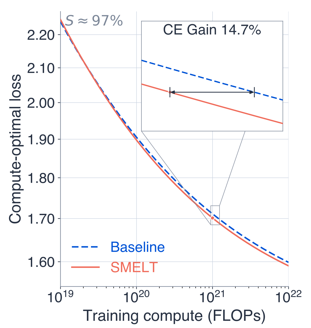
Both architectures get their own six-coefficient Chinchilla-style fit (), and SMELT's capacity exponent ( vs. Baseline's ) and data exponent ( vs. ) are both larger — its reducible loss drops faster with both compute and data. Converted to a compute-efficiency figure (the fraction of training compute SMELT saves at matched loss, the standard algorithmic-progress metric from Hernandez & Brown):
| SMELT budget | S≈85% | S≈95% | S≈97% |
|---|---|---|---|
| 10^20 FLOPs | 10.0% [1,22] | 7.8% [3,15] | 6.8% [4,14] |
| 10^21 FLOPs | 18.0% [8,28] | 15.8% [10,25] | 14.7% [8,25] |
| 10^22 FLOPs† | 23.5% [8,42] | 20.9% [0,48] | 19.6% [0,51] |
Bracketed ranges are 95% cell-bootstrap intervals (2,000 resamples of the twelve sparse grid cells). † Extrapolated beyond the fitted compute window (1.3×10^19-2.2×10^21 FLOPs) — treat this row as a projection, not a measurement. Hardware is not disclosed anywhere in the paper — SMELT trains on "a proprietary Transformer family whose complete architecture and training stack cannot be released" (Appendix A), so every number here is FLOPs, never wall-clock, and there's no accelerator to check the FLOPs figure against.
This is the actual headline, and it's worth stating plainly against the framing every parameter-matched paper invites: looping still wins after you pay for the FLOPs, but the win shrinks from "a 50M model beats a 150M one" (virtual logic depth's number) to a 6.8-18.0% training-compute discount. Real. Compounding — the gap widens as compute grows, because SMELT's fitted frontier exponent ( vs. Baseline's ) is larger. But it is not the free lunch the "no extra parameters" framing implies once you're the one holding the compute budget rather than the parameter budget.
One number that doesn't move much: tokens-per-parameter at the compute-optimal split lands within 6% of the Baseline's at every sparsity level (both architectures want roughly the same split between model size and data, 56-91 tokens/param depending on sparsity — both well above Chinchilla's dense-model ~20). SMELT's saving comes from reaching lower loss at the same allocation, not from spending the budget differently.
Downstream, and where the second visit spends its attention
Validation loss isn't the benchmark that matters to a user, so the paper checks whether the gain survives contact with real evaluations. It wins DCLM Completion in all 96 matched pairs, DCLM Core in 83 of 96, and MMLU in 29 of 30 pairs where the Baseline clears chance by 10+ points — and critically, fitting a sigmoid calibration from validation loss to each benchmark (following Bhagia et al.'s task-scaling method) shows SMELT's downstream score exceeds what its validation-loss improvement alone would predict, with the excess growing at larger scale. Code benefits most among training domains (20.4% CE Gain vs. 14.8% for Web), and the advantage concentrates on long samples (1.52× the gain on the four longest length buckets vs. the four shortest) and grows with more in-context examples — on Dyck-language bracket matching specifically, SMELT reaches 29.8% accuracy at 32 shots against the Baseline's 26.4%, and the gap widens with shot count rather than plateauing.
The mechanistic probe behind that ICL number is the most interesting part of the paper's second half: tracing what the second visit through a shared layer actually does differently. Query and key vectors stay nearly unchanged between visits (cosine similarity 0.89-0.93) — the model keeps its retrieval coordinates — while value vectors diverge more (0.65-0.74), and the attention sink at the sequence-start token nearly vanishes on the second pass (segment-start mass falls from 0.60 to 0.02 on a Dyck-language case study, redistributing onto the actual answer tokens). The second visit isn't recomputing from scratch or discarding the first; it's redirecting attention away from the sink and toward content, using coordinates the first visit already established. That's a genuine mechanistic account, though the paper is careful to call it "a descriptive starting point" toward a causal one, not the causal account itself.
Two more checks against the same bar
The full-bandwidth transformer takes a different attack on the same depth problem, and is unusually honest about the cost. Covered in full here: rather than looping a block, it feeds the discarded top-layer hidden state back into the next decoding step through a gated fusion, keeping the KV cache and objective untouched. What's relevant to this piece is that the paper defines its own token-equivalent compute metric explicitly — a two-pass training batch costs 2× a standard batch, a three-pass batch 3× — and reports it plainly in a table rather than hiding it:
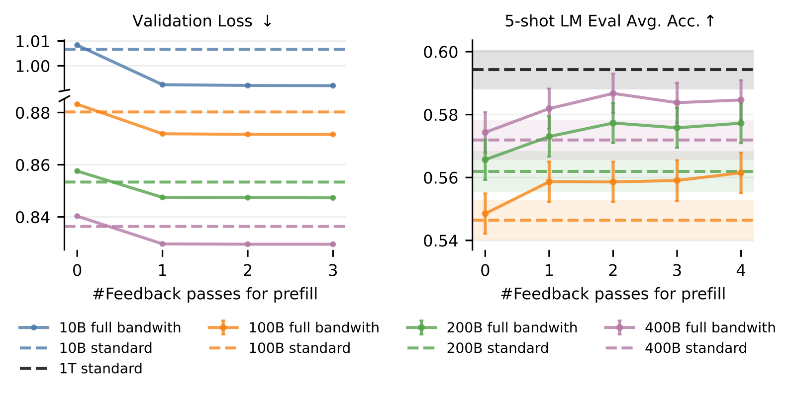
Their headline claim — matching standard transformers trained on roughly 1.5× more tokens — holds up better than most under scrutiny: their own table shows a 100B-token run costs 150B token-equivalent training compute (a 75/25 mix of one-pass and three-pass training batches) and still comes in under a 200B-token Baseline's 200B compute, so the training-compute side of the comparison is, if anything, conservative in the paper's own favor. What it doesn't fully account for is the inference-time cost: the "reaches the 200B-token baseline" comparisons apply two additional fused prefill passes at evaluation time, a real per-query compute cost the raw-token chart above doesn't show. This is compute relocated from training to serving, not compute avoided — a legitimate trade, but a different one than SMELT's, which matches both training and inference cost simultaneously. Sebastian Raschka's write-up on this paper (see below) names a limitation the authors don't fully close either: nobody tested whether a conventionally scaled-up transformer — more blocks, not a feedback loop — produces the same shortened-reasoning-trace effect the paper credits to latent feedback specifically.
Nanbeige4.2-3B is the existence proof, and it inherits the confound rather than escaping it. Covered in depth here: a shipped, open-weight 3B-non-embedding model, pretrained from scratch on 28T tokens with a full-stack loop ×2, that reports beating Qwen3.5-9B and Gemma4-12B across most agent and reasoning benchmarks. Two things are worth being precise about. First, Nanbeige's own report is honest, in the same sentence virtual logic depth never wrote: the loop "retains approximately 75% of the token efficiency" relative to an unlooped model — a plain admission that FLOPs are not matched, stated as a design tradeoff rather than buried. Second, and this is the point that matters: Nanbeige's comparison against Qwen3.5-9B and Gemma4-12B is not parameter-matched, FLOPs-matched, or KV-cache-matched — it's a 3B model claiming to beat 9-12B ones on every axis at once, with none of them controlled. Applying the same first-order FLOPs-per-token estimate this site used for virtual logic depth ( effective depth multiplier) to Nanbeige's stated 3B non-embedding parameters and loop count 2: per-token compute lands closer to what a single-pass ~6B dense model would spend, not 3B. That's still smaller than Qwen3.5-9B or Gemma4-12B assumed dense and single-pass — so the "beats a bigger model" claim plausibly survives a rough compute check — but it's a 6B-ish-compute model beating 9-12B-parameter ones, not a 3B one, and the gap is real but roughly half of what the raw parameter counts alone suggest. This estimate is mine, not the paper's, and it assumes both competitor models are dense; I could not verify that from public information, so treat it as illustrative, matching the disclosure this site gave the same calculation in virtual logic depth. Nanbeige also found, independently, that sharing the KV cache across loop passes to halve the memory cost consistently hurt performance — so the shipped model keeps the full, non-shared cache, meaning its serving KV footprint is not matched to its competitors' either. Nobody ran the SMELT-style three-budget match on Nanbeige, and given it isn't MoE, the SMELT recipe's specific lever (narrow width, add experts) isn't even available to it. It's a real production model with a real capability win. It is not evidence that the win survives compute-matching, because nobody has checked.
What Raschka's framing gets right, and the Astra rumor
Sebastian Raschka's September 9 write-up covers this same territory — the mechanics of block reuse, the Universal Transformer lineage's adaptive halting (a per-position, learned stopping probability, dating to Dehghani et al. 2019), and the Mixture-of-Recursions-style routing that assigns each token its own loop depth rather than a single architecture-wide . That routed-depth axis is worth flagging precisely because SMELT doesn't touch it — is fixed for every token, and the paper lists per-token adaptive depth explicitly as future work ("[relaxing] the simplest form of looping... token-level adaptive recursion depth"). Whether letting easy tokens exit after one pass and hard tokens loop twice would change the compute-matched picture is a real open question this paper doesn't address. Raschka covers this same landscape and lands SMELT and the full-bandwidth transformer specifically as the compute-matched frontier. His summary of SMELT's number is accurate: "SMELT requires about 6.8-18% less training compute to reach the same validation loss within the studied compute range" — which is the right way to state it, bounded to the studied range rather than extrapolated.
His treatment of the GPT-6 Astra rumor is careful in a way worth naming explicitly, since this site has covered that rumor before and takes the same position: The Information reported, from unnamed sources, that Astra uses "recurrent depth" or "looped transformers." Raschka states plainly that this is "still just a rumor or scoop, with no official confirmation," and reports OpenAI chief scientist Jakub Pachocki's actual statement — that the computation-graph depth of Astra is "within a factor of two" of GPT-4 — which does not confirm a looped architecture at all; a deeper conventional stack would say the same thing. Raschka goes on to offer his own opinion that Astra likely does use some form of looping, on the strength of the rumor plus the technique's demonstrated promise — that's a stated opinion, clearly marked as one, not a claim of fact. Nothing in this article depends on Astra using looped transformers, and nothing here treats the rumor as more than a rumor.
What to trust, and what to hold loosely
The take
Virtual logic depth's own criticism — that the field's headline "reasoning without extra parameters" numbers were never checked against the FLOPs those extra passes actually cost — turns out to be exactly right, and SMELT is the first paper to close all three of the budgets that matter (FLOPs, parameters, KV cache) at once and check. The honest answer sits between the two extremes a reader might have guessed: looping is neither the free lunch the parameter-matched literature implied, nor a mirage that evaporates once you pay for it. It's a real 6.8-18.0% training-compute discount that compounds as the budget grows, purchased by a specific, MoE-only trick — trade width for depth, and use the expert pool to buy back the parameters the narrower width gave up. That trick doesn't transfer to a dense model the way Nanbeige ships one, which is why Nanbeige's real production win and SMELT's controlled one are not the same kind of evidence, even though they point the same direction. And it's a training-time story specifically — the full-bandwidth transformer's complementary result, that a small amount of inference-time compute can substitute for a larger training-time budget, is a genuinely different lever, honestly accounted for in tokens even where the inference side of its own ledger is thinner. Three papers, no shared citations between them, converging on the same conclusion from three different budgets: looping is a real architectural lever, not just relabeled scale — just a smaller one, once somebody bothers to check.
Sources: SMELT: Scaling Laws for Compute-Matched MoE Looped Transformers (arXiv 2609.01343v1, Wang, Zhang, Luo, Wu, Liu, Liu, Huang, Yan, Li, 1 September 2026), read in full via the arXiv HTML rendering; Full-bandwidth transformer (arXiv 2608.08888, 9 August 2026, CC BY 4.0), previously covered in full; the Nanbeige4.2-3B technical report, previously covered in full; and Sebastian Raschka's September 9, 2026 write-up. All tables and figures reproduce the source papers' own numbers exactly except where marked illustrative; illustrative FLOPs estimates (the naive-loop bars in the interactive above, and the Nanbeige compute-equivalence figure) are first-order approximations this site computed from each paper's own stated relations, not numbers the papers report themselves.