2026-09-09 · 26 min · kv-cache · inference-optimization · llm · systems · explainer
Every production LLM stack that routes between model sizes pays the same tax on every swap. Cascade a cheap draft up to a bigger model when confidence is low, escalate mid-conversation, or route a query to whichever size fits its difficulty — the pattern this site has covered from the draft-model side already — and the receiving model has to re-prefill the entire accumulated context from scratch before it can say a word. Prefill cost scales with model size and prompt length, and it's the forward pass that populates the KV cache — the thing that makes generation possible at all. Prefix caching helps, but only within one model. The moment you swap sizes, everything the first model computed about the conversation so far is thrown away and repaid at the second model's price.
Cross-Model KV Cache Transfer in LLM Families (Heo, Shafipour, Zhao, Golub, Kamani, Borkar, Chandran, Zardoshti, Darvish Rouhani — NVIDIA, arXiv 2608.03893) asks whether that repayment is actually necessary. If a source model's KV cache and a target model's KV cache are related in a learnable way, the target could decode directly from a mapped version of the source's cache and skip prefill entirely. The paper's finding is that this relationship is largely linear — linear enough that a closed-form ridge regression, fit on 500 short documents with no backpropagation at all, recovers most of a target model's standalone accuracy on four of the six pairs it tests. The other two collapse. Both halves of that sentence are the story.
| Paper | Cross-Model KV Cache Transfer in LLM Families: A Closed-Form Linear Mapping for Prefill Reuse |
| Constraint | Matched-KV: source and target must share KV head count and per-head dimension (, ) |
| Test families | Qwen3 (8B/14B → 32B), Llama 3.1 (8B → 70B), Ministral 3 (3B/8B → 8B/14B) — six pairs, three families |
| The mapper | Per-head ridge regression, closed-form, no gradient-based training, fit from 500 FineWeb-Edu sequences × 1,024 tokens |
| Headline result | 73–98% of standalone accuracy on four of six pairs; two collapse to 42–44% (11–15% floor-normalized) |
| Speed | 2.7–25× faster than re-prefill across seven pairs and ten context lengths — mapper wins all 70 measured cells |
| Code | Not released at time of writing |
The pipeline
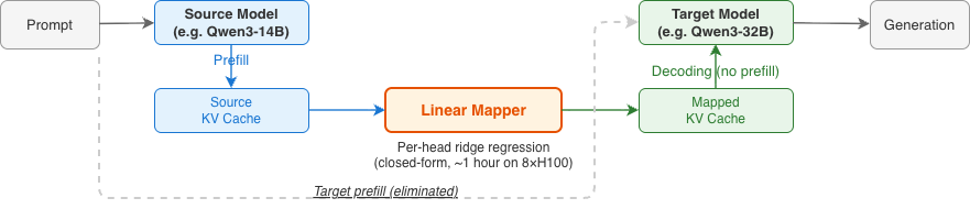
The receiver never runs its own forward pass over the prompt. It only ever sees the mapped cache. Two things have to be true for this to work at all: the mapping has to exist, and it has to be cheap enough to fit that skipping prefill is still a net win. Section 2.3 of the paper is about the first question.
Why a linear map works at all
Define matched KV: source and target share KV head count and per-head dimension , even when layer count, hidden size, or total parameters differ. The paper restricts itself entirely to matched-KV pairs — it's the precondition for asking whether a linear map from one model's per-token key/value vectors to another's can work at all, since without it the vectors don't even live in comparably-shaped spaces.
On Qwen3, fitting a single ordinary-least-squares regression from one source layer's keys to one target layer's keys already explains real variance:
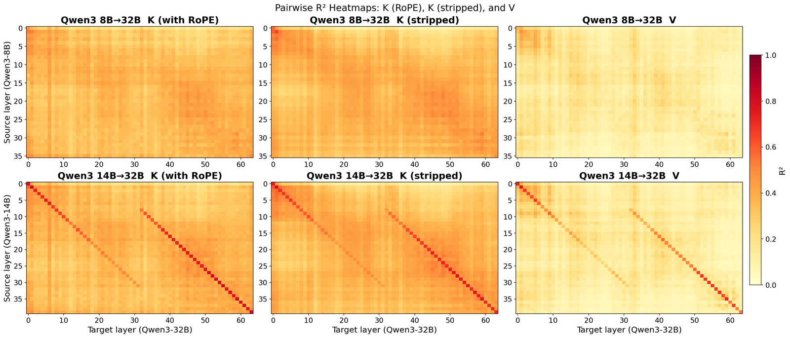
The headline "56%... 79%" numbers from the abstract are Appendix C's Table 7, and they're worth seeing as a real progression rather than two isolated percentages — this is on Qwen3 14B → 32B, averaged across target heads:
| Source layers used () | K | V |
|---|---|---|
| 1 (best single layer) | 55.7% | 32.5% |
| 8 | 79.1% | 65.4% |
| all (40) | 84.5% | 76.5% |
Two things fall out of this table. First, keys are consistently more predictable than values — roughly a 20-point gap at every , which the paper attributes to values carrying no positional structure to exploit and generally encoding more idiosyncratic per-token content. Second, the jump from to is where almost all of the gain is (79.1% is 94% of the way to the ceiling of 84.5%) — a single source layer is nowhere near sufficient, but a handful of them, concatenated, capture most of what all forty would. That's the empirical basis for the mapper's cross-layer selection step below, not an arbitrary design choice.
The mapper: three steps, one closed-form solve
For each target (layer , head ) pair, the mapper does three things.
1. Cross-layer source selection. Rank every source layer by its single-source, head-averaged against this specific target layer (that's exactly the heatmap above), keep the top , and concatenate their key/value features into one wide input vector. is swept per pair over and fixed to whichever value maximizes benchmark accuracy — Qwen3 14B → 32B lands on , Llama 3.1 8B → 70B needs before its curve flattens.
2. Content-space mapping — strip RoPE before fitting. The KV cache stores keys after rotary position encoding has already been applied: . Fitting a linear map directly on those rotated keys ties the learned weights to the exact 1,024-token position distribution seen during calibration — reasonable at short context, but it means the fit has implicitly memorized "what position 400 looks like" rather than "what this token's content looks like." Since is an orthogonal rotation matrix, inverting it is exact and free, so the mapper strips it from both sides before fitting, learns the map in position-free content space, and re-applies the target's own RoPE at inference:
This is the part that makes one fitted mapper reusable at any context length the target's RoPE supports, not just the 1,024 tokens it was calibrated on — a map fit only on rotated keys would be implicitly bound to that one length. Values carry no positional encoding, so they map directly, with no rotate/strip/re-rotate step at all.
3. Ridge regression, closed form. Stack calibration tokens into a design matrix and targets , center both, and solve once:
with throughout — small enough not to bias the fit, large enough to keep invertible when pushes the feature dimension into the tens of thousands and the selected layers are, by construction, correlated with each other. No gradient descent anywhere in this pipeline. As pseudocode, the whole thing (Eqs. 2–6, K side; V is identical minus the RoPE step):
# Fitting one target (layer l, head h)'s K-mapper. Run independently for
# every (layer, head) pair -- no parameters shared across heads or between K/V.
def fit_target_head(target_layer, head, source_layers, k, lam=0.01):
    # 1. Cross-layer source selection: rank every source layer by single-source
    #    R^2 against this target layer, keep the top k, concatenate their keys.
    scored = [(l, r2_single_source(l, target_layer, head)) for l in source_layers]
    top_k = [l for l, _ in sorted(scored, key=lambda t: -t[1])[:k]]

    # 2. Content-space mapping: strip RoPE from source AND target keys before
    #    fitting, so the map is learned position-free.
    X = concat([strip_rope(K_source[l][head]) for l in top_k])   # [N, k * n_kv_s * d_h_s]
    Y = strip_rope(K_target[target_layer][head])                  # [N, d_h_t]

    # 3. Closed-form ridge -- one linear solve, no backprop, no epochs.
    Xc, Yc = X - X.mean(0), Y - Y.mean(0)
    W = inv(Xc.T @ Xc + lam * I) @ Xc.T @ Yc
    b = Y.mean(0) - X.mean(0) @ W
    return W, b, top_k

def apply_mapper(W, b, top_k, source_cache, head, positions, target_rope):
    X = concat([strip_rope(source_cache.K[l][head]) for l in top_k])
    K_hat_content = X @ W + b                       # position-free
    return apply_rope(K_hat_content, positions, target_rope)  # re-rotate into target space
Calibration is 500 FineWeb-Edu sequences of 1,024 tokens, stride-4 subsampled to roughly 128K token-level observations per target head. Fitting the entire mapper for one pair — every layer, every head, K and V — takes 47–87 minutes on a single 8×H100 node, with zero gradient steps: Qwen3 8B → 32B is the fastest at ~47 min, Ministral 8B → 14B the slowest at ~87 min. That speed is real and is the whole selling point of "closed-form": no training run, no loss curve, no hyperparameter search beyond sweeping one integer ().
Does it work? Four pairs out of six
Four of six matched-KV pairs land in the 73–98% band the abstract leads with; Qwen3 14B → 32B is close enough to standalone that its ARC-C column even edges past 100% (noise, not the mapper beating the target’s own cache). The two Ministral pairs targeting 14B sit apart, near 42–44% — and every pair’s diamonds show GSM8K pulling hardest below the bar, worst on Llama 3.1 8B → 70B (18.2%) and near-total collapse on both Ministral 14B targets (1.6–3.2%).
The full per-pair table (paper, Table 1) — retention is transfer accuracy divided by the target's own standalone accuracy; floor-normalized retention is , which places each benchmark's chance floor at 0% and the target's own accuracy at 100%:
| Family | Pair () | Avg | Avg (floor-norm.) | ARC-C | HellaSwag | WinoGrande | MMLU | GSM8K |
|---|---|---|---|---|---|---|---|---|
| — | Chance floor | — | — | 25% | 25% | 50% | 25% | ≈0% |
| Qwen3 | 14B → 32B (8) | 97.6% | 96.3% | 101.0% | 97.6% | 98.5% | 95.0% | 95.6% |
| Qwen3 | 8B → 32B (12) | 87.5% | 80.7% | 94.0% | 95.2% | 91.0% | 88.5% | 68.8% |
| Ministral 3 | 3B → 8B (all) | 76.2% | 65.9% | 90.6% | 93.3% | 91.3% | 69.4% | 36.6% |
| Llama 3.1 | 8B → 70B (20) | 72.8% | 62.9% | 90.9% | 94.4% | 87.1% | 73.3% | 18.2% |
| Ministral 3 | 3B → 14B (20) | 44.2% | 14.7% | 43.6% | 68.0% | 74.0% | 32.0% | 3.2% |
| Ministral 3 | 8B → 14B (12) | 41.6% | 11.1% | 40.7% | 58.7% | 74.2% | 32.7% | 1.6% |
The abstract's own framing is worth reading literally: "Surprisingly, across six pairs in three families, this linear mapper retains 73–98% of the receiver's standalone-prefill accuracy on four pairs, while two degrade sharply." That's the honest version — four of six, not six of six — and it's still the right headline to lead with, because a training-free linear map recovering most of prefill quality on any pair at all is a real result. The two failures aren't a subtle miss, either. Ministral 3B → 14B and 8B → 14B both target the same 14B checkpoint, and Table 13's raw numbers show what "44% avg" actually looks like per benchmark: 8B → 14B's mapped MMLU accuracy is 25.25% against a 25% chance floor and a 77.33% standalone target — floor-normalized, that's +0.5%, indistinguishable from a coin flip. The same pair's floor-normalized MMLU on the 3B source is −0.5% — at or fractionally below chance. Both 14B-targeting pairs' GSM8K retention rounds to 1.6% and 3.2%. This isn't "worse than standalone." On MMLU and GSM8K specifically, the mapped model has stopped doing the task.
Does the paper explain the two failures? Not fully
The natural next question is why the 14B target specifically breaks. Section 4.5 investigates this, and the answer is more interesting than "it's a bigger gap" — because the size of the gap turns out not to be the explanation.
The a priori metric you'd reach for is calibration — if the linear fit is good, transfer should be good. It doesn't hold up across pairs. Llama 3.1 8B → 70B fits ridge at and retains 94% HellaSwag small-to-large — but only 37% in the reverse, large-to-small direction, at the same calibration fit quality. Ministral 3B → 8B fits at the identical and retains 93% in both directions. Two pairs, same , wildly different downstream outcomes. measures how well the mapper reconstructs each channel on average; it says nothing about whether the reconstruction error lands somewhere attention actually reads.
What does correlate is attention-output cosine similarity — comparing the actual attention output the target computes from mapped KV against the attention output from its own ground-truth KV, averaged over layers and heads. Across 12 pair-evaluations (six pairs, both directions), cosine correlates with HellaSwag retention at Pearson ; calibration manages only — technically the wrong sign. The mechanism the paper proposes is error concentration: project the mapper's key error onto the target's own query matrix's singular vectors (weighted by squared singular value) and value error onto the ground-truth attention weights — concentration above 1 means residual error lands where attention actually reads; below 1 means it lands where attention ignores it. A worse-looking fit that happens to misplace its error in attention-irrelevant directions can outperform a better-looking fit that concentrates its error exactly where the query looks.
That's a real, useful diagnostic — but notice what it doesn't do: it explains that the two Ministral pairs concentrate error badly, not why those two pairs specifically do. The paper is direct about this gap in its own future-work section: "Beyond architecture, training-data overlap, fine-tuning recipe, and other non-architectural factors may also influence transferability. We leave systematic study of these to future work." So: no, not fully. The paper has a correlate (attention-output cosine) and a partial fix (below), but not a diagnosed cause for why the 14B target is the hard one.
One more thing worth checking, since the paper doesn't frame it this way: parameter ratio doesn't predict the split either. Llama 3.1 8B → 70B — the largest size gap tested at 8.75× — is a clean success (72.8% avg). Ministral 8B → 14B — the smallest size gap tested at just 1.75× — is one of the two failures (41.6% avg). If anything, the failure pairs are the ones with the smaller jumps. Whatever is different about matched-KV transfer into this particular 14B checkpoint, it isn't simply "the target is too much bigger."
The MLP fixes the failures — and quietly retires "closed-form"
Section 4.4 tests the obvious follow-up: replace ridge with a small nonlinear MLP, same MSE loss, same calibration data, only the mapper's functional form changes. On the pairs where ridge already works, the MLP is a wash or slightly worse. On the two failures, it's transformative:
| Pair | Ridge (HellaSwag) | MLP (HellaSwag) | |
|---|---|---|---|
| Qwen3 14B → 32B | 97.6% | 97.3% | −0.3 pp |
| Ministral 3B → 8B | 93.3% | 91.8% | −1.5 pp |
| Ministral 3B → 14B | 68.0% | 92.3% | +24.3 pp |
| Ministral 8B → 14B | 58.7% | 95.5% | +36.8 pp |
The abstract's "up to +37 pp" is the top of a 12.5-point-wide range (+24.3 to +36.8), and both ends matter: even the smaller gain moves a pair from clearly failing to comfortably above 90%. Table 4 in the paper ties this to the same error-concentration mechanism above — on the two failure pairs, switching to the MLP drops K-concentration by roughly 2.3–2.7 and lifts attention-output cosine by roughly 0.41–0.48, redistributing residual error away from the directions the target's queries actually read. On the pairs ridge already handles, the same swap barely moves either quantity, and sometimes moves both in the "right" direction while HellaSwag retention still slips slightly — evidence that redistributing error only pays off once misplaced error was large enough to bind in the first place.
Here's the tension worth naming plainly: the paper's central pitch is a mapper that's closed-form and training-free — no backprop anywhere. The MLP that rescues exactly the pairs that most need rescuing is neither. It's a genuine multilayer perceptron — per (target layer, head, K or V), two 1,024-unit ReLU hidden layers, trained with Adam at learning rate for 20 epochs, batch size 4,096, MSE loss (Appendix E). For Qwen3-32B as a target that's layers KV heads 2 (K and V) independently-trained small networks, each requiring actual gradient descent. The paper reports ridge's fitting time precisely (47–87 minutes, zero backprop) and never states the MLP's — an honest gap worth flagging rather than guessing at a number. What's certain is the shape of the tradeoff: linear ridge stays sufficient exactly where the cross-model KV relationship is already linear, and the moment it isn't, the fix that works also gives up the "closed-form" property that was the paper's headline framing.
The speed math: 2.7–25×, and no crossover in the tested range
Both curves rise with context length, but re-prefill rises faster — the gap between re-prefill and the mapper widens from 4× at 64 tokens to 25× at 32,768, all within the range the paper actually measured. Nowhere in that range does re-prefill catch up: across all seven pairs and ten sequence lengths in Appendix G, the mapper is faster in every one of 70 measured cells — there is no observed crossover to find, only a gap that keeps growing with context length and, separately, with how many source layers a pair’s selected k concatenates (a bigger k means a heavier per-token matmul, which is part of why Llama 3.1 8B → 70B’s k=20 tops out lower than this pair’s k=8 despite transferring into a much larger target).
Table 5 gives exact latency at three context lengths for Qwen3 14B ↔ 32B, at each direction's selected :
| Seq len | Mapper (ms) | Re-prefill (ms) | Speedup | Mapper (ms) | Re-prefill (ms) | Speedup |
|---|---|---|---|---|---|---|
| small → large (k=8) | large → small (k=20) | |||||
| 64 | 14.0 | 61.7 | 4× | 11.6 | 39.2 | 3× |
| 8K | 67.8 | 1,154.8 | 17× | 101.9 | 501.0 | 5× |
| 32K | 277.6 | 6,975.3 | 25× | 427.1 | 2,952.7 | 7× |
The mapper is a per-layer batched matrix multiply against the source's cache — no attention operator, no quadratic term, cost grows close to linearly with sequence length. Re-prefill runs the target's actual transformer body, attention included, and its cost grows faster. That's the whole mechanism behind "2.7–25×": it isn't one fixed multiplier, it's a gap between a near-linear curve and a superlinear one, and the ratio widens the longer the context gets — visible directly in the interactive above (drag the slider; the two curves separate more the further right you go).
Appendix G's extended sweep (Table 16) runs this across all seven measured pairs and ten context lengths from 64 to 32,768 tokens, and states its own scope plainly: "the mapper is faster in every one of the 70 cells." No pair, no length, no direction in the tested range favors re-prefill — there's no crossover to report, only where the gap is smallest (short context, small pairs) and largest (long context, the sharpest-fitting pair):
| Direction | Family | Pair () | Transfer @ 32K | Re-prefill @ 32K | Speedup range (64–32K) |
|---|---|---|---|---|---|
| S→L | Qwen3 | 14B → 32B (8) | 278 ms | 6,975 ms | 4.4–25.1× |
| S→L | Qwen3 | 8B → 32B (12) | 392 ms | 6,975 ms | 4.3–17.8× |
| S→L | Llama 3.1 | 8B → 70B (20) | 777 ms | 11,562 ms | 4.5–14.9× |
| S→L | Ministral 3 | 3B → 14B (20) | 396 ms | 2,465 ms | 3.8–6.2× |
| S→L | Ministral 3 | 3B → 8B (all) | 438 ms | 1,764 ms | 2.7–4.0× |
| L→S | Qwen3 | 32B → 14B (20) | 427 ms | 2,953 ms | 3.3–6.9× |
| L→S | Llama 3.1 | 70B → 8B (10) | 216 ms | 1,652 ms | 2.8–7.6× |
The abstract's low end, 2.7×, belongs to Ministral 3B → 8B at short context — the smallest parameter ratio among the small-to-large pairs (2.67×) and the smallest target, so re-prefill was never going to be that expensive to begin with. The high end, 25.1×, is Qwen3 14B → 32B at 32K — the sharpest-fitting pair (highest calibration , smallest ) transferring into the context length where re-prefill's cost has grown the most. Context length is the dominant lever, but it isn't the only one: notice Llama 3.1 8B → 70B tops out lower (14.9×) than Qwen3 14B → 32B (25.1×) despite transferring into a far larger target — because Llama's harder-to-fit pair needs concatenated source layers against Qwen3's , and a bigger means a proportionally heavier per-token matmul for the mapper itself. Speedup is a function of both curves, not just the target's re-prefill cost.
Matched-KV: how restrictive is this, really?
Every pair the paper tests is matched-KV by construction (Appendix D, Table 10) — the paper doesn't
claim otherwise, and explicitly lists "matched-KV is empirical" and "we do not test mismatched-KV
pairs" among its own limitations. The open question is how much of a real family this constraint
actually covers. I pulled config.json directly from the Hugging Face Hub for the model pairs the
paper names, plus a few adjacent releases it doesn't test, to check:
| Model | KV heads | Head dim | Layers | Matches Qwen3-32B? |
|---|---|---|---|---|
| Qwen3-0.6B | 8 | 128 | 28 | yes |
| Qwen3-1.7B | 8 | 128 | 28 | yes |
| Qwen3-4B | 8 | 128 | 36 | yes |
| Qwen3-8B | 8 | 128 | 36 | yes |
| Qwen3-14B | 8 | 128 | 40 | yes |
| Qwen3-32B | 8 | 128 | 64 | — (target) |
| Qwen3-30B-A3B (MoE) | 4 | 128 | 48 | no |
| Qwen3-235B-A22B (MoE) | 4 | 128 | 94 | no |
Every dense Qwen3 checkpoint from 0.6B to 32B shares 8 KV heads and a 128 head dimension — the constraint is essentially free across the whole dense ladder, which is a more generous result than "matched-KV" sounds like it should be. But Qwen3's own MoE checkpoints, sold under the identical "Qwen3" name, use 4 KV heads instead of 8. Cascading from a cheap dense model up to the flagship Qwen3-235B-A22B MoE — arguably the single most realistic cost-quality-cascade scenario the paper's own introduction motivates — is exactly the kind of swap this method cannot serve, without anyone having changed model families at all.
| Model | KV heads | Head dim | Matches Llama-3.1-8B/70B? |
|---|---|---|---|
| Llama-3.1-8B | 8 | 128 | — (source) |
| Llama-3.1-70B | 8 | 128 | — (target) |
| Llama-3.2-1B | 8 | 64 | no |
| Llama-3.2-3B | 8 | 128 | yes |
Llama tells the same story from a different angle: 3.1's 8B and 70B match each other, and 3.2's 3B continues the pattern — but 3.2's 1B model quietly halves its head dimension to 64, breaking from the rest of the lineage it's marketed alongside. Ministral 3, for what it's worth, checks out clean across all three sizes the paper tests: 3B, 8B, and 14B all report 8 KV heads and a 128 head dimension. So the real answer is pair-specific, not family-specific: matched-KV holds reliably within a single dense architecture's own size ladder, and breaks the moment a swap crosses into a different attention shape released under the same brand name — MoE variants being the most common way that happens in practice.
- architecture
- Qwen3ForCausalLM
- task
- text-generation
- library
- transformers
- license
- apache-2.0
- safetensors
- 8 shards
- largest file
- 3.96 GB
- files
- 18
- downloads
- 1.7M
- likes
- 463
The paper's best-retention source model — 8 KV heads, 128 head dim, 40 layers, matched with Qwen3-32B below.
repo last modified 2025-07-26
- architecture
- Qwen3ForCausalLM
- task
- text-generation
- library
- transformers
- license
- apache-2.0
- safetensors
- 17 shards
- largest file
- 3.96 GB
- files
- 27
- downloads
- 5.2M
- likes
- 743
The paper's best-retention target — same KV head count and head dimension as 14B, which is the matched-KV precondition, not a coincidence.
repo last modified 2025-07-26
The calibration set is tiny — and it's actually ablated
500 sequences of 1,024 tokens is a genuinely small calibration set for fitting over a billion mapper parameters, and it's a fair thing to be suspicious of. The paper runs the sensitivity sweep, on Qwen3 14B → 32B / HellaSwag (Table 8):
| Sweep | Setting | HellaSwag | vs. production |
|---|---|---|---|
| (N=500, FineWeb) | 0 | 80.86 | +0.13 |
| 1e-4 | 80.88 | +0.15 | |
| 0.01 (production) | 80.73 | — | |
| 0.1 | 79.75 | −0.98 | |
| 1 | 64.94 | −15.79 | |
| (=0.01, FineWeb) | 50 | 79.09 | −1.64 |
| 100 | 79.72 | −1.01 | |
| 200 | 80.44 | −0.29 | |
| 500 (production) | 80.73 | — | |
| 1000 | 80.89 | +0.16 | |
| Domain (=0.01, N=500) | CodeAlpaca | 75.46 | −5.24 |
| Wikipedia | 79.65 | −1.05 | |
| FineWeb-Edu (production) | 80.70 | — |
Both and have wide, flat regions — the per-head system is over-determined enough that even (a twentieth of production) stays within 1.6 points, and the curve visibly flattens by . Regularization only collapses at , an order of magnitude past where the ridge penalty starts dominating the least-squares objective outright. So no, this isn't fragile to sample count or regularization strength.
Domain is the one axis with a real, if modest, cost, and the paper extends the check across seven log-likelihood benchmarks by domain (Table 9):
| Benchmark | Register | FineWeb-Edu | Wikipedia | CodeAlpaca |
|---|---|---|---|---|
| HellaSwag | commonsense | 80.70 | 79.65 (98.7%) | 75.46 (93.5%) |
| MMLU | broad knowledge | 78.07 | 78.05 (100.0%) | 78.13 (100.1%) |
| ARC-Challenge | hard science QA | 61.60 | 61.26 (99.5%) | 56.23 (91.3%) |
| ARC-Easy | easy science QA | 83.63 | 83.08 (99.4%) | 80.43 (96.2%) |
| PIQA | physical commonsense | 80.79 | 80.79 (100.0%) | 79.49 (98.4%) |
| BoolQ | reading comprehension | 87.31 | 85.72 (98.2%) | 88.50 (101.4%) |
| WinoGrande | coreference | 68.98 | 69.22 (100.3%) | 62.27 (90.3%) |
| Mean | 77.30 | 76.82 (99.4%) | 74.36 (95.9%) |
Retention never drops below 90% in any single cell, but the two substitute corpora fail differently: Wikipedia stays within noise everywhere (99.4% mean, tight spread), while CodeAlpaca averages a real but small 95.9% and ranges over 11.1 points — matching FineWeb-Edu almost exactly on MMLU and BoolQ while costing the most on coreference and hard science QA, the benchmarks furthest from CodeAlpaca's own register. That's calibration-domain mismatch showing up exactly where you'd expect it to: not uniformly, but concentrated on the tasks least like the calibration text.
The limitations section is upfront about the boundary on all of this: every number above is on one pair (Qwen3 14B → 32B, the easiest one), and "neither substitution separates subject matter from register, so the sweep does not bound calibration confined to a single field such as medicine or law." A calibration set that works fine mixing FineWeb-Edu, Wikipedia, and CodeAlpaca hasn't been shown to work for a deployment whose actual traffic is one narrow domain.
Multi-turn handoff: does drift compound?
The realistic deployment isn't one swap — it's a conversation that alternates between source and target across many turns, escalating and de-escalating as difficulty changes. The paper checks this on Qwen3 14B ↔ 32B with CoQA, 100 conversations of roughly 15 turns each, defining drift at turn as the F1 gap between the target's standalone accuracy and the mapper's accuracy at that same turn. Small-to-large drift widens by 1.7 pp from turn 1 to turn 10; large-to-small drift grows roughly linearly at 0.33 pp per turn. Both are small within a ten-turn window — nothing that reads as cascading failure — though the paper is careful to note the linear large-to-small trend would keep accumulating over a much longer session than the one it tested.
What this doesn't establish
Collecting the paper's own stated limitations in one place, since several of them qualify results used as headlines elsewhere in this piece: matched-KV is an empirical property of the six tested pairs, not a structural guarantee of the method, and mismatched-KV transfer is untested entirely. Per-pair is selected on the same log-likelihood benchmarks the paper then reports accuracy on — Appendix H bounds the resulting optimism at "at most 2.49 pp," which is small but not zero, and a proper held-out selection is explicitly not what was done. And the whole method is scoped to within-family transfer over dense, full-attention models; hybrid attention and attention-recurrent architectures (state-space hybrids like Nemotron 3) are named as out of scope and left to future work, alongside cross-family transfer (Qwen3 → Llama 3.1, say) being entirely open.
None of that erases the core result. A closed-form, gradient-free linear map recovering 73–98% of standalone accuracy on four of six real matched-KV pairs, at 2.7–25× the latency of re-prefill, is a genuinely useful building block for exactly the swap-heavy serving patterns the introduction motivates. It's just a building block with a documented, roughly-1-in-3 failure rate on the pairs tested so far, a fix for those failures that isn't closed-form anymore, and a real-world matched-KV footprint narrower than "within a family" implies once MoE variants enter the picture.
Related on this site: TurboQuant attacks the same KV-cache capacity problem from the compression side rather than the reuse side; SparDA takes KV-cache pressure as a given and optimizes what to fetch and when; and EAGLE-3 and the AMD vLLM speculative-decoding benchmarks cover the other place a draft/target model pair shows up in serving — accelerating one model's decoding rather than skipping another model's prefill. How LLM inference works is the background piece on why prefill and the KV cache exist in the first place.
Built on Cross-Model KV Cache Transfer in LLM Families: A Closed-Form Linear Mapping for Prefill
Reuse (Heo, Shafipour, Zhao, Golub, Kamani, Borkar, Chandran,
Zardoshti, Darvish Rouhani; NVIDIA, 2026). Figures fetched from
arxiv.org/html/2608.03893v1/figures/ and flattened onto white. Matched-KV configuration numbers
independently verified against each model's config.json on the Hugging Face Hub.