2026-09-08 · 23 min · sparse-attention · kv-cache · long-context · inference · attention
Why read this
Solidtop 85%Explains the one-layer-ahead Forecast projection and pulls apart its three speedups by baseline; the +6.5 reasoning gain rests on two 30-problem AIME sets.
- Original analysis
- A new technique
- Open code or weights
Inference & servingNeeds datacenter GPUsResearch paper
How this was scored
- Is it new?
- 2 of 3: A real new idea, method or capability
- Can I trust it?
- 2 of 3: Measures key facts from files, code or configs
- Can I run it?
- 2 of 3: Open code or weights with real limits
- Will I understand it?
- 2 of 3: Mechanism from first principles with figures
- Can I act on it?
- 1 of 3: General advice
- Will it last?
- 1 of 3: Relevant for months
- Does it affect many?
- 1 of 3: A specialist community
- Only here?
- 2 of 3: A teardown or measurement few others did
Score 58 of 100, ranked 376 of 577 rated articles. Each question is answered 0–3 by hand, and a 3 is rare. How articles are scored
Sparse attention is sold as the fix for long-context inference: instead of every query attending to every past token, a selector picks a handful of relevant blocks and attention runs only over those. That drops the attention FLOPs from to . It does not, on its own, fix two things SparDA's authors call out directly in their own abstract:
- The KV cache still grows with . Sparse attention reads less of the cache per step, but the cache itself — every key and value ever produced — still has to live somewhere. Once it stops fitting in GPU memory, the standard move is to offload it to CPU RAM and fetch selected blocks over PCIe on demand. PCIe is much slower than GPU memory bandwidth, so that fetch becomes the new bottleneck.
- Selection is still . Picking which blocks matter means scoring every candidate block against the query, and that scoring cost doesn't shrink just because the attention that follows it did. At long enough context, selection can cost more than the sparse attention it's selecting for.
SparDA (Yaosheng Fu, Guangxuan Xiao, Xin Dong, Song Han, Oreste Villa — NVIDIA, MIT, and co-authors whose current affiliations span Thinking Machines Lab and ByteDance Seed, per the paper's own footnote marking work done while at NVIDIA; arXiv 2606.04511) attacks both problems with one architectural change: a fourth per-layer projection, alongside Q, K, and V, called the Forecast.
| Paper | SparDA: Sparse Decoupled Attention for Efficient Long-Context LLM Inference |
| Builds on | InfLLM-V2 block-sparse attention (initial + local + top-k selected blocks) |
| The change | A 4th projection, Forecast , predicts layer 's selected blocks from layer |
| Forecast indexer | One Forecast head per GQA group (not per query head); softmax dropped entirely |
| Added params | 33.5M on an 8B model — 0.41% |
| Training | Only the Forecast projections, by KL-matching the original selector's block-attention distribution |
| Test models | MiniCPM4.1-8B and NOSA-8B, both already sparse-pretrained on InfLLM-V2-style attention |
| Accuracy | Matches or slightly improves over the sparse baseline (exact per-benchmark deltas below) |
| Efficiency | Up to 1.25× prefill, 1.7× decode over sparse+offload; up to 5.3× decode throughput over non-offload sparse — three different baselines |
| Code | NVlabs/SparDA |
The problem InfLLM-V2 leaves on the table
SparDA is built on top of InfLLM-V2 (Zhao et al., ICLR 2026), which is architecturally representative of block-sparse attention generally — the same initial-block / local-window / top-k-selected-block shape shared by NSA, MoBA, and QUEST. For a query at position , layer attends only to:
Keys get mean-pooled into compressed representations, the query scores against those, and the top-k blocks by score go into . This is the same story this site has covered before: decode is memory-bandwidth-bound, one query token per step, so anything that shrinks how much of the KV cache a step has to touch pays off directly. SparDA's summary of GQA-aware attention variants gives the fuller picture of what MHA, MQA, GQA and sparse selection are each trading away to pay down that bill, and TurboQuant covers the other lever on the same problem — compressing what's in the cache rather than reading less of it.
The move this paper is really about isn't sparsity itself. It's who decides what to select, and when. In InfLLM-V2's baseline, the same query that will run attention also drives the top-k selection, in the same layer, back to back — selection sits directly on attention's critical path, and it can't start early because it depends on , which doesn't exist until layer 's linear projection has already run.
That's not a novel observation to this site. DeepSeek Sparse Attention already decouples selection from the query at the token level, using a small "lightning indexer" instead of the full attention query to score candidates — and both Hy4 preview's IndexCache and GLM-5.3's indexer_types reuse push the idea further by sharing one layer's index across several neighboring layers, on the theory that adjacent layers attend to similar things. SparDA's contribution is doing the same decoupling at block granularity instead of token granularity, and — the part DSA-style indexers don't do — using the decoupling to open a prefetch window, not just a cheaper index.
The fourth projection
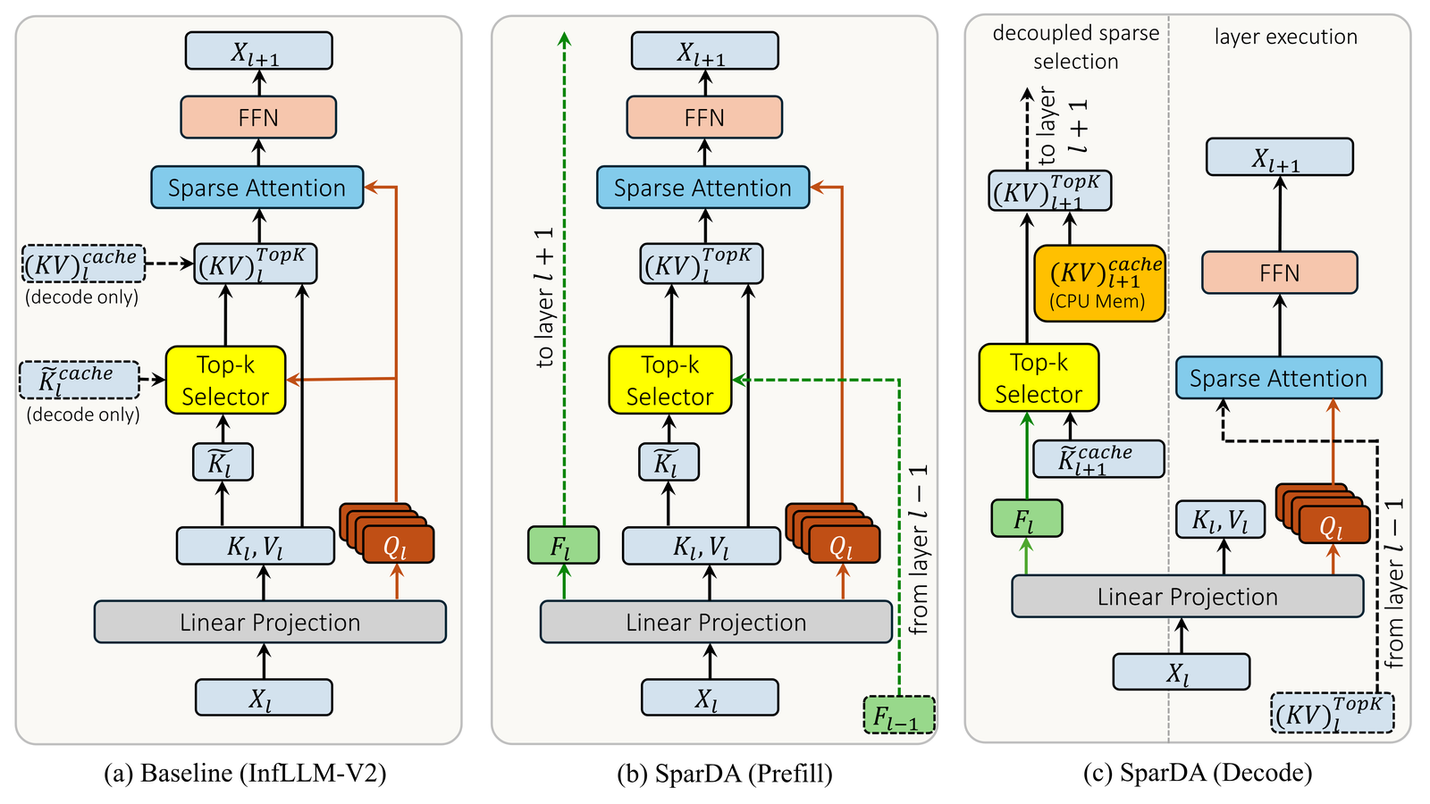
The linear projection in every layer now produces four tensors instead of three:
— the Forecast — scores against layer 's compressed keys and selects that next layer's attended blocks:
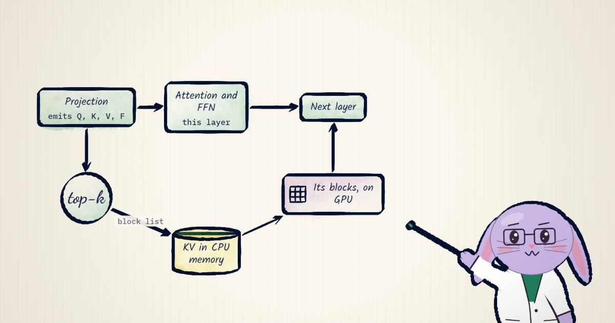
Layer 's own query is still what actually runs attention — Forecast only picks which blocks get attended, one layer before they're needed. That one-layer offset is the entire trick. Because exists right after layer 's projection — before attention, before the FFN — the runtime knows which CPU-resident KV blocks layer will want while layer is still busy computing. It can launch the CPU-to-GPU transfer immediately and let it run concurrently with layer 's attention and FFN, on a dedicated CUDA stream through a persistent Unified-Virtual-Addressing kernel built for exactly this (Section 4.3 of the paper — the kernel detail itself isn't the story here, the scheduling opportunity it enables is).
Written out as pseudocode, adapted directly from the paper's own Algorithm 1 (prefill step, Appendix A) — the fourth projection and the one-layer-ahead handoff are the whole change:
# One SparDA layer, prefill (Algorithm 1). phi_l is the model's existing
# linear projection, just widened by one small head group for F_l.
def sparda_layer_prefill(X_l, F_prev, layer_l):
    Q_l, K_l, V_l, F_l = phi_l(X_l)              # Eq. 3 -- F_l is new

    # F_prev = F_{l-1}, produced one layer ago, selects THIS layer's blocks.
    B_l = B_init | B_local | top_k(F_prev @ K_compressed[layer_l].T, k)

    O_l = attention(Q_l, K_l[B_l], V_l[B_l])       # Eq. 5 -- ordinary Q_l
    X_next = ffn_l(O_l)

    # F_l is handed forward, unused by this layer's own attention -- it
    # exists only to pick layer l+1's blocks (Eq. 4).
    return X_next, F_l
Two regimes matter differently here, and the paper is explicit about the split (this is the central caveat of the whole piece, so it's worth stating before the numbers below make it easy to miss): during prefill, every key is already resident on GPU. There's nothing to prefetch — the entire benefit of decoupled selection in prefill is that Forecast's compact indexer is cheaper to compute than the original multi-head selector, not that anything gets hidden behind a transfer. During decode, the KV cache is offloaded to CPU, and that's when the lookahead prefetch actually does its job — hiding a PCIe transfer that would otherwise stall the next layer. Read every speedup number below with that distinction in mind; conflating the two regimes is the single easiest way to overstate what this paper shows.
The decode-time version is Algorithm 2 in the paper, and the two-CUDA-stream structure is what makes the overlap in the diagram above real rather than aspirational — one stream keeps computing while a second, dedicated stream (the persistent UVA kernel, Section 4.3) handles the transfer:
# One SparDA layer, decode -- one new token (Algorithm 2). `compute_stream`
# runs attention/FFN as normal; `prefetch_stream` is the dedicated stream
# driving the persistent UVA kernel, launched once and left running.
def sparda_layer_decode(X_l, B_l, layer_l):
    Q_l, K_l, V_l, F_l = phi_l(X_l)
    kv_cache[layer_l].append(K_l, V_l)
    k_compressed_cache[layer_l].update_incremental(kv_cache[layer_l])

    # Pick l+1's blocks NOW -- before this layer has even attended -- and
    # hand the transfer to the prefetch stream immediately, asynchronously.
    B_next = B_init | B_local | top_k(F_l @ k_compressed_cache[layer_l + 1].T, k)
    prefetch_stream.launch_async(fetch(B_next, src="CPU pinned", dst="GPU"))

    # B_l's own fetch was launched a full layer ago, while layer l-1 was
    # still executing -- by now it has usually had time to finish.
    compute_stream.wait(prefetch_stream, until=B_l)
    O_l = attention(Q_l, kv_cache[layer_l][B_l], kv_cache[layer_l][B_l])
    X_next = ffn_l(O_l)
    return X_next, B_next
The one line worth staring at is wait(prefetch_stream, until=B_l): in the synchronous
baseline that wait is where every layer stalls, because the fetch it's waiting on hasn't even
been launched yet. Here it's usually a no-op, because the transfer had an entire previous layer's
worth of compute to finish in.
One Forecast head per GQA group
Decoupling selection from the query buys a second thing beyond timing: it frees the selector from having to match attention's head layout at all. In the baseline, every one of the query heads in a GQA group scores the candidate blocks independently, the per-head scores get summed into a shared group score, and then softmax runs before top-k ranking — the same three-stage compression pipeline InfLLM-V2, MoBA, and SeerAttention all use. That's score matmuls and a softmax, every layer, every step.
Forecast doesn't need to preserve per-query-head structure, because nothing downstream cares which query head "owns" a selection — attention still runs full-width against regardless. So SparDA's GQA implementation collapses this to one Forecast head per GQA group (one per KV head, not per query head) and drops the softmax normalization outright, since there's no per-head summation left to normalize. This is the block-level version of what DeepSeek's lightning indexer already does at the token level — SparDA's own related-work section says so directly — extended to block-sparse attention and, unlike a same-layer indexer, computed one layer ahead so its output feeds a prefetch instead of only a cheaper score.
Side by side, the baseline's three-stage compression (Section 3.1) and the Forecast indexer (Section 4.1) reduce to this — the softmax isn't skipped as an approximation, there's structurally nothing left for it to normalize once the per-head sum disappears:
# Baseline selector (InfLLM-V2 / NSA / MoBA shape). G query heads share one
# GQA group; every one of them scores every candidate block.
def baseline_select(Q_heads, K_compressed, k):      # Q_heads: G query heads
    scores = [Q_h @ K_compressed.T for Q_h in Q_heads]   # G score matmuls
    shared = sum(scores)                                  # sum across heads
    weights = softmax(shared / sqrt(d))                   # normalize, still paid
    return top_k(weights, k)

# SparDA's Forecast indexer (Sec. 4.1). One head per GQA group -- one per KV
# head, not per query head -- so there's no per-head sum left to normalize.
def forecast_select(F_group, K_compressed, k):       # F_group: 1 head
    scores = F_group @ K_compressed.T                 # 1 score matmul
    return top_k(scores, k)                            # ranking only
Both test models share a top-k budget of 96 blocks at block size 64 (with a 32-window, stride-16 compression kernel for the pooled keys) — MiniCPM4.1-8B spends 32 of those blocks on a 2,048-token local window, NOSA-8B spends 16 blocks (1,024 tokens) on its local window plus 24 blocks on query-aware top-k selection specifically, following its own architecture (Appendix C). None of that changes the shape of the selection-cost argument above; it's the config the paper's measured numbers were run at.
Training: distilling the selector you already have
SparDA is designed to be dropped onto a model that's already sparse-pretrained — MiniCPM4.1-8B and NOSA-8B both ship with a working InfLLM-V2-style selector before SparDA touches them. Adding SparDA means training only the Forecast projections (the main one plus a separate layer-0 projection, since layer 0 has no previous-layer Forecast to inherit) — the base model's weights, including the original selector, are frozen.
The training target is the original selector's own block-attention distribution — specifically the shared importance score before its final max-pooling step, computed at a finer compression granularity than inference uses, because max-pooling throws away exactly the ranking detail the indexer needs to learn from. Forecast is trained to match that distribution via KL divergence, computed over a top-k-restricted, renormalized set (the target's own top-k blocks individually, everything else pooled into one "rest" bucket) — the same training shape DeepSeek DSA uses for its indexer, minus DSA's full-model sparse pretraining stage, since these base models are sparse already.
The objective, from Equations 6–7 — only the Forecast projections have gradients flowing into them here, everything else (including the target-producing selector) is frozen:
# Eq. 6: target comes from the ORIGINAL selector -- G query heads summed,
# scored against a FINER compression grid than inference uses (kernel 2,
# stride 1, vs. the standard 32/16) because max-pooling throws away the
# ranking detail the indexer needs to learn from.
S_target = sum(softmax(Q[l, h] @ K_fine_target[l].T / tau) for h in group)

# Predicted score: the previous layer's Forecast, no GQA summation needed.
S_pred = softmax(F[l - 1] @ K_pred[l].T / tau)       # K_pred: standard 32/16 grid

# Eq. 7: KL over a top-k-restricted, (k+1)-dim renormalized distribution --
# the target's own top-k blocks kept individually, everything else pooled
# into one "rest" bucket, so out-of-set blocks still get a small gradient.
selected = top_k(S_target, k)                 # after causal mask, minus init/local
S_target_bar = restrict_and_renormalize(S_target, selected)
S_pred_bar = restrict_and_renormalize(S_pred, selected)
loss = sum(kl_div(S_target_bar[l], S_pred_bar[l]) for l in all_layers)
# Only S_pred_bar's parameters (the Forecast projections) get gradients.Does it hold accuracy? The real per-benchmark deltas
Aggregated across HELMET, LongBench, RULER, and a long-reasoning suite (MATH-500, AIME 2024, AIME 2025), SparDA edges the sparse baseline on both models — but "matches or slightly improves" hides real texture worth pulling apart. The full aggregate table (paper Table 1):
MiniCPM4.1-8B (evaluated at its 64K native max)
| Method | HELMET | LongBench | RULER | Reasoning | Avg |
|---|---|---|---|---|---|
| Dense | 41.7 | 44.8 | 85.3 | 82.3 | 63.5 |
| Sparse | 38.9 | 45.0 | 78.2 | 83.6 | 61.4 |
| InfiniGen | 33.5 | 45.1 | 68.4 | 83.7 | 57.7 |
| SparDA | 38.3 | 45.1 | 78.7 | 84.7 | 61.7 |
NOSA-8B (32K native max)
| Method | HELMET | LongBench | RULER | Reasoning | Avg |
|---|---|---|---|---|---|
| Dense | 39.3 | 42.5 | 86.2 | 41.6 | 52.4 |
| Sparse | 32.2 | 42.4 | 72.2 | 50.7 | 49.4 |
| InfiniGen | 28.1 | 41.6 | 65.2 | 47.6 | 45.6 |
| SparDA | 33.4 | 42.3 | 73.9 | 57.2 | 51.7 |
Reading down each SparDA row against Sparse: MiniCPM4.1-8B goes +0.3 average, with RULER +0.5 and reasoning +1.1 pulling it up while HELMET actually drops 0.6 (38.9 → 38.3) and LongBench is essentially flat — a net win, not a win everywhere. NOSA-8B's larger +2.3 average is worth tracing to its source before repeating it as one number: HELMET +1.2, RULER +1.7, and reasoning +6.5 (50.7 → 57.2) — the single biggest number in either table, and the one worth the most scrutiny, because "reasoning" is an average of three very differently-sized datasets:
| Dataset (NOSA-8B, GPT-5.2 judge) | Dense | Sparse | InfiniGen | SparDA | Δ vs Sparse |
|---|---|---|---|---|---|
| MATH-500 (500 problems) | 68.2 | 72.2 | 72.8 | 71.6 | −0.6 |
| AIME 2024 (30 problems) | 43.3 | 40.0 | 40.0 | 46.7 | +6.7 |
| AIME 2025 (30 problems) | 13.3 | 40.0 | 30.0 | 53.3 | +13.3 |
| Average | 41.6 | 50.7 | 47.6 | 57.2 | +6.5 |
The +6.5 average is driven almost entirely by two 30-question competition-math sets, where a handful of flipped answers moves the score by several points — and on the one dataset with real sample size (MATH-500, 500 problems), SparDA is marginally behind the sparse baseline it's supposedly matching. That doesn't make the AIME gains noise; it means treating "+6.5 on NOSA-8B long reasoning" as a settled, model-general result — rather than one model, one category, substantially two 30-problem benchmarks — reads more confidence into it than the data supports. For comparison, MiniCPM4.1-8B's own reasoning suite moves by a much smaller +1.1 (Table 14 in the paper's appendix runs the same per-dataset breakdown for it).
Length generalization on RULER holds up better as a trend — SparDA beats Sparse at every extended length on both models (paper Table 2):
| Model | Method | 32K | 64K | 96K | 128K |
|---|---|---|---|---|---|
| MiniCPM4.1-8B | Sparse | 86.1 | 78.2 | 68.7 | 67.7 |
| MiniCPM4.1-8B | SparDA | 87.6 | 78.7 | 70.8 | 68.8 |
| NOSA-8B | Sparse | 72.2 | 56.6 | 48.8 | 40.7 |
| NOSA-8B | SparDA | 73.9 | 60.5 | 52.9 | 45.0 |
On NOSA-8B the gap widens steadily with length — +1.7 at 32K, +3.9 at 64K, +4.1 at 96K, +4.3 at 128K — suggesting the learned Forecast generalizes at least as well as the training-free baseline selector even past the lengths it was trained at; MiniCPM4.1-8B's gap is smaller and less monotonic (+1.5, +0.5, +2.1, +1.1).
For context on the comparison itself: InfiniGen — the closest prior lookahead-prefetch method, which uses raw hidden states as a proxy for future attention instead of a trained Forecast — degrades noticeably on both models (57.7 average on MiniCPM4.1-8B, 45.6 on NOSA-8B, both below the plain sparse baseline in the first table above). The paper's explanation matches the mechanism: hidden-state similarity across adjacent layers is the assumption InfiniGen leans on, and it "does not always hold."
Three speedups, three different baselines
This is where the paper's abstract compresses three genuinely different measurements into three adjacent numbers, and it's worth naming the baseline each one is actually measured against before citing any of them:
| Headline number | Measured against | Regime | MiniCPM4.1-8B | NOSA-8B |
|---|---|---|---|---|
| "1.25× prefill" | Sparse with offload, same batch | prefill, 128K | 1.25× | 1.16× |
| — | Dense, no offload, same batch | prefill, 128K | 2.11× | 1.40× |
| "1.7× decode" | Sparse with offload, same batch | decode, 128K, best batch (B8) | 1.69× | 1.40× |
| "5.3× throughput" | Sparse, no offload, each at its own peak feasible batch | decode, 128K | 5.28× (B64 vs B4) | 8.16× (B64 vs B4)† |
†Computed here from Table 4's own NOSA-8B numbers, not stated by the paper as a headline figure — the paper reports "up to 5.28×... on MiniCPM4.1-8B" and separately says NOSA-8B shows lower speedups, which the table itself doesn't bear out for this particular comparison (more below).
Offload barely matters in prefill — every key is already on GPU there — so "1.25× prefill" is really "the Forecast indexer is cheaper to run than the original multi-head selector." The full prefill table (paper Table 3, tokens/sec, H100) makes the trend across context length visible:
| Model | Method | 32K | 64K | 96K | 128K |
|---|---|---|---|---|---|
| MiniCPM4.1-8B | Dense (no offload) | 20,388.3 | 13,673.7 | 10,228.3 | 8,085.8 |
| MiniCPM4.1-8B | Sparse (offload) | 18,548.4 | 16,254.4 | 14,707.7 | 13,661.8 |
| MiniCPM4.1-8B | SparDA | 19,845.6 | 18,379.5 | 17,715.2 | 17,087.6 |
| NOSA-8B | Dense (no offload) | 20,438.9 | 13,701.0 | 10,244.1 | 8,118.0 |
| NOSA-8B | Sparse (offload) | 12,778.3 | 11,359.2 | 10,448.5 | 9,805.2 |
| NOSA-8B | SparDA | 13,456.0 | 12,386.1 | 11,807.3 | 11,332.7 |
Dense leads at short sequences — no selection overhead to pay at all — but its quadratic scaling gives that up by 64K on both models. SparDA leads Sparse from 64K onward on MiniCPM4.1-8B and from 96K onward on NOSA-8B, which is consistent with selection cost being the thing that's shrinking: it only starts to dominate at long enough context for the saving to show up.
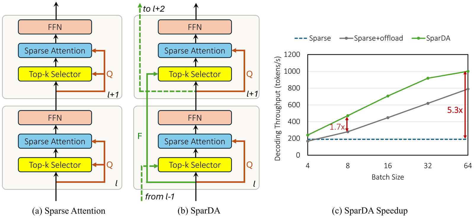
Decode throughput at 128K, across the full batch sweep, is where the offload-vs-no-offload distinction earns its keep (paper Table 4, tokens/sec, H100; "–" is an out-of-memory cell, not a zero):
| Method | B4 | B8 | B16 | B32 | B64 | B128 |
|---|---|---|---|---|---|---|
| MiniCPM4.1-8B | ||||||
| Dense, no offload | 108.6 | – | – | – | – | – |
| Sparse, no offload | 189.5 | – | – | – | – | – |
| Sparse, offload | 167.8 | 279.5 | 447.9 | 618.6 | 788.9 | – |
| InfiniGen | 51.8 | 66.5 | 85.6 | 117.5 | – | – |
| SparDA | 240.2 | 471.2 | 705.3 | 899.2 | 1,000.1 | – |
| NOSA-8B | ||||||
| Dense, no offload | 108.4 | – | – | – | – | – |
| Sparse, no offload | 179.3 | – | – | – | – | – |
| Sparse, offload | 173.2 | 285.4 | 529.2 | 898.7 | 1,298.3 | – |
| InfiniGen | 77.5 | 105.2 | 131.7 | 166.9 | – | – |
| SparDA | 219.0 | 399.3 | 735.0 | 1,127.0 | 1,463.3 | – |
Both non-offload rows (Dense†, Sparse†) OOM past batch 4 at this context length — the entire KV cache has to sit on GPU, so there's no room left to grow the batch. That's the "5.3×" claim's real mechanism: SparDA's peak MiniCPM4.1-8B throughput (1,000.1 tok/s at B64) against non-offload Sparse's only achievable point (189.5 tok/s at B4) is 5.28×, and against non-offload Dense (108.6) it's 9.21× — both numbers the paper states explicitly for MiniCPM4.1-8B. It's worth flagging what the same table implies for the other model, since the paper doesn't spell it out the same way: it says "NOSA-8B shows lower speedups because its query-agnostic eviction head already reduces KV fetch traffic" — true for the iso-batch decode number (1.40× vs. 1.69×) — but running NOSA-8B's own peak-feasible numbers from this table (1,463.3 at B64 over 179.3 at B4) gives 8.16×, higher than MiniCPM4.1-8B's 5.28×, not lower. Both figures come from the same published table; the "lower speedups" sentence appears to describe the matched-batch comparison, not the peak-batch one it's positioned next to.
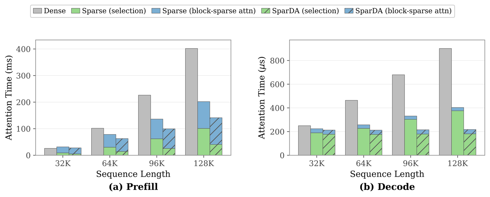
That's the mechanism the attention-time breakdown above shows directly: on MiniCPM4.1-8B at batch 4, per-layer attention time splits into block-selection (green) and block-sparse-attention (blue). In prefill, selection grows with sequence length and becomes comparable to attention itself by 128K; SparDA cuts that selection cost up to 2.50× while leaving the attention computation itself about the same. In decode, with only one query token per step, block-sparse attention is cheap and selection dominates instead — Sparse's selection cost keeps growing with context length, while SparDA's Forecast indexer stays nearly flat, cutting the overhead more than 2× at 128K. The interactive above works from the same Table 4 decode-throughput numbers as the table and Figure 1(c) here, at finer batch-size granularity and with the non-offload OOM ceiling made explicit.
What this doesn't fix
SparDA doesn't change the sparse attention pattern itself, and it says so plainly: it's "not itself a sparse attention method," it's a selection-and-scheduling layer bolted onto one that already exists. The efficiency wins are real and specific — cheaper selection everywhere, and hidden PCIe latency specifically in the offloaded-decode regime — but they come with the ceiling above (bounded by the base selector's own accuracy), a sample-size caveat on the single largest accuracy headline, and a scope limit the authors state themselves: two 8B, already sparse-pretrained models, on a block-sparse backbone. Whether the same one-layer-ahead trick holds up on DSA's token-level indexer, on DeepSeek-V4's Compressed Sparse Attention, or at the scale those models actually run at, is explicitly future work, not something this paper measured.
Built on SparDA: Sparse Decoupled Attention for Efficient Long-Context LLM Inference
(Yaosheng Fu, Guangxuan Xiao, Xin Dong, Song Han, Oreste Villa; NVIDIA, MIT, Thinking Machines Lab,
ByteDance Seed, 2026). Code at NVlabs/SparDA. Figures rendered
from the paper's own LaTeXML SVGs at arxiv.org/html/2606.04511v1/.