Squeeze3D: a borrowed 3D generator as the decoder, and what its 2,187x is made of

md json mcp

2026-10-07 · 23 min · 3d · compression · point-cloud · representation-learning · self-supervised-learning · synthetic-data

Why read this

Essentialtop 10%

Explains Squeeze3D's latent bridge and Gram loss via the Barlow Twins duality, then rebuilds each ratio from files and weights and finds three errors.

Original, source-checked analysis
Interactive explanations
A lasting reference

3D & spatialNeeds a workstation GPUMITResearch paper

How this was scored

Is it new?: 2 of 3: A real new idea, method or capability
Can I trust it?: 3 of 3: Reproduces the headline result, or shows from primary files it is wrong
Can I run it?: 2 of 3: Open code or weights with real limits
Will I understand it?: 3 of 3: Mechanism carried by interactives built from real code or data
Can I act on it?: 2 of 3: A concrete recipe, numbers or comparison
Will it last?: 2 of 3: A reference for a year or more
Does it affect many?: 1 of 3: A specialist community
Only here?: 3 of 3: The only place this analysis exists

Score 80 of 100, ranked 20 of 454 rated articles. Each question is answered 0–3 by hand, and a 3 is rare. How articles are scored

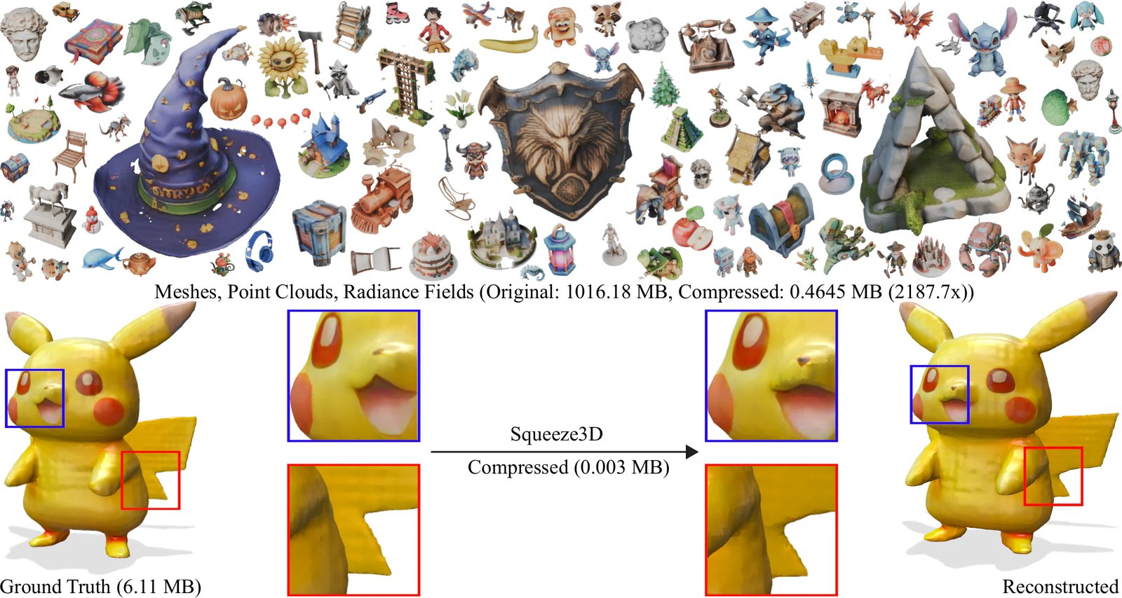
I spend a lot of my working week moving point clouds and meshes around, so a post that says "meshes: 2,187x compression" gets my attention the way a benchmark with no hardware listed does. Rishit Dagli posted Squeeze3D on X with three ratios: 2,187x for meshes, 58.5x for point clouds, 619x for radiance fields. The thread framed it less as a codec and more as a question: how do you bridge the latent spaces of two models that were never trained together, with no reconstruction loss at all, only a loss in latent space plus what he called a dimension-wise contrastive loss?

That framing turned out to be the more interesting half. The paper, arXiv 2506.07932, is now the TMLR camera-ready (v2, 28 September 2026), and the code and weights are public under MIT. I read all three. The latent bridge is simple and the regulariser that keeps it from collapsing has a tidy explanation the paper doesn't give. The headline ratios are a different story. They are arithmetic on file sizes, and the files they divide by are worth looking at.

A collage of dozens of textured 3D assets above a close-up comparison of a yellow cartoon mouse mesh before and after compression, labelled 6.11 MB and 0.003 MB. — The paper's teaser: a 6.11 MB textured mesh and its reconstruction from a 0.003 MB code. The reconstruction is InstantMesh regenerating the object, not a decoded copy of the original file (Squeeze3D paper, Figure 1).

Borrow a decoder, train only the plumbing

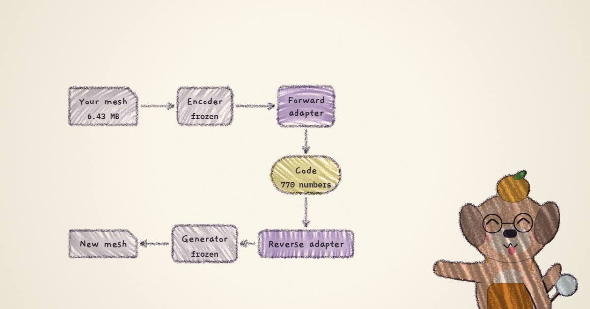
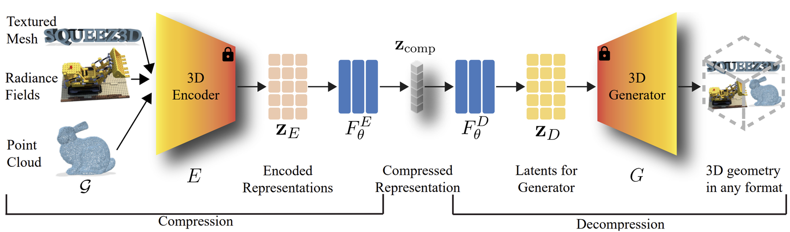
A 3D generator such as InstantMesh, Shap-E or LION has already learned a prior over plausible objects. Give its decoder the right latent and it produces a whole textured mesh. Squeeze3D's bet is that this latent can be reached from a short code, and that the code can be computed from any object you already have.

Three frozen or trained pieces do the work:

a pre-trained 3D encoder $E$ that reads the object you want to compress (MeshAnything for meshes, PointNet++ for point clouds, NeRF-MAE for radiance fields);
a forward mapping network $F^E_\theta$ that squeezes the encoder's latent into a short code $z_\text{comp}$ of width $d_C$ ;
a reverse mapping network $F^D_\theta$ that expands that code into the latent the generator's decoder $G$ expects.

Compression is $z_\text{comp} = F^E_\theta(E(\mathcal{G}))$ . Decompression is $G(F^D_\theta(z_\text{comp}))$ . The encoder and the generator never change. Only the two adapters train, and one trained pair serves every object for that encoder, generator and code width.

Pipeline diagram: a mesh, a radiance field and a point cloud enter a locked 3D encoder, its encoded representation passes through a forward mapping network to a small compressed vector, then a reverse mapping network produces latents for a locked 3D generator, which outputs 3D geometry. — Compression runs the frozen encoder and the forward mapping network; decompression runs the reverse mapping network and the frozen generator. The padlocks mark the parts that never train (Squeeze3D paper, Figure 2).

In the code the two adapters are one module. For meshes it is LTOrtho in squeeze3d/models/mlp.py, and its forward pass is short enough to quote whole (lines 391-406):

identity = self.fc1(x)          # 263,168 inputs (257 x 1024) -> d_C
x = self.ln1(identity)
x = F.gelu(x)
x = self.dropout1(x)
 
x = self.fc2(x)                 # d_C -> d_C
mid = x                         # the tensor the Gram loss sees and the scripts save
x = self.ln2(x + identity)
x = F.gelu(x)
x = self.dropout2(x)
 
x = self.fc3(x)                 # d_C -> generator latent (983,040 for InstantMesh)
return x, mid

The forward adapter is fc1 and fc2; the reverse adapter is ln2 and fc3. For InstantMesh, configs/mesh_ma_instantmesh.py sets hidden_size to 770 and the output to 3 * 80 * 64 * 64, the triplane that InstantMesh's own decoder turns into a mesh. So the code is 770 float32 numbers, 3,080 bytes, and the target is 983,040 numbers. Notice the residual: what fc3 sees is the sum of mid and identity. That detail comes back later.

The point-cloud version (LTpcOrtho, lines 500-576) is a 12-layer MLP of uniform width $d_C$ from PointNet++'s 1,024-number global feature to LION's 8,320-number latent (128 global plus 8,192 local), with the code taken from the middle layer. The radiance-field version (LTNeRFOrtho, lines 657-735) is a 3D convolutional encoder-decoder whose bottleneck is 24 channels on a $10^3$ grid, 24,000 numbers.

Training on latents the generator made itself

The training data is the clever bit, and it is what makes "no reconstruction loss" possible. You need pairs: an encoder latent for some object, and the generator latent that produces the same object. Nobody has those pairs for real objects, because nobody knows which generator latent produces a given artist mesh. So the paper runs the generator forward. Sample a condition (a rendered Objaverse image for InstantMesh and OpenLRM, a prompt for Shap-E, plain noise for LION), keep the generator latent, decode it to a mesh, and run that mesh through the encoder. Now you have an exact pair, by construction.

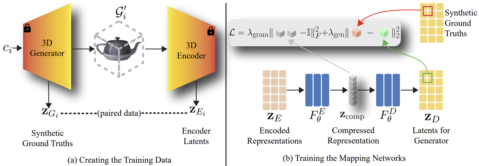
Two-panel diagram. Left: a condition goes into a locked 3D generator, which produces a teapot; the teapot goes through a locked 3D encoder; the generator's latent and the encoder's latent form a paired example. Right: the encoder latent passes through the forward network to a compressed code and the reverse network to generator latents; the loss compares those latents with the synthetic ground truth and adds a Gram term on the compressed code. — Left, the paired data: every training object is one the generator made, so its generator latent is known exactly. Right, the loss: a Gram term on the code plus an MSE between predicted and true generator latents (Squeeze3D paper, Figure 3).

The training step in squeeze3d/launch_training.py only ever compares latents. The criterion is nn.MSELoss() (line 831), applied between the reverse network's output and the stored generator latent, plus the Gram term. The decoder is never called during training. No mesh is extracted, no image is rendered, no Chamfer distance is computed.

That matters for three reasons, in rising order of importance.

It is cheap. Table 12 puts the InstantMesh mapping at 12 GPU-hours of training plus 20 hours of data creation, on one RTX 4090 or up to four H100s. Rendering 36 views or running marching cubes inside the loop would multiply that.

It sidesteps differentiability. These decoders were never built to be backpropagated through for someone else's objective: InstantMesh extracts a mesh from a triplane, LION runs a point-cloud VAE decoder, Shap-E renders an implicit function. The repo still carries a half-built attempt at decoder supervision for Shap-E (lines 369-400), and it shows why people avoid it. The images are rendered under torch.no_grad(), the tensor is detach()ed and given a fresh requires_grad, and then the loss becomes loss * outputs.sum() * 0 + loss. That last line attaches the graph only so backward() doesn't complain; the gradient reaching the mapping network is exactly zero. It is off by default (use_decoder_supervision=False), and the paper reports only the latent-only runs.

The deepest reason is the one in the thread: if you can bridge latent spaces with latent losses alone, the method doesn't care what is downstream. Any frozen encoder, any frozen generator, as long as the generator can be sampled to make pairs. That's the JEPA instinct, predict in representation space rather than in pixels, applied to plumbing between two models instead of to learning one. The JEPA-Anything and NextLat write-ups on this site come at the same instinct from the other side.

The cost is that a latent MSE weighs every coordinate of the generator latent equally, while the decoder does not. Some triplane channels barely move the output and others move it a lot, and the loss can't tell them apart. The paper doesn't measure how much this costs, and with the decoder out of the loop there is no signal that could.

The Gram loss is Barlow Twins wearing the other matrix

With MSE alone, the paper reports that the codes collapse onto a few directions. Stack a batch of $B$ codes into $Z \in \mathbb{R}^{B \times d_C}$ and the singular values fall off steeply, the correlation matrix $Z^\top Z / B$ fills with large off-diagonal entries, and the effective dimension

d_\text{eff} = \frac{\left(\sum_i \lambda_i\right)^2}{\sum_i \lambda_i^2}

(their Eq. 5, with $\lambda_i$ the eigenvalues) sits far below $d_C$ . For a compressor that is waste: you are paying for 770 floats and using a handful.

The fix is the term the paper calls the Gram loss. Here it is as the code computes it, launch_training.py lines 81-100:

def ortho_loss(criterion, outputs, targets, b):
    primary_loss = criterion(outputs, targets)          # latent MSE
 
    b_normalized = b / (torch.norm(b, dim=1, keepdim=True) + 1e-8)
    gram_matrix = torch.matmul(b_normalized, b_normalized.transpose(0, 1))
    target = torch.eye(b.shape[0], device=b.device)
    loss = torch.mean((gram_matrix - target) ** 2)
 
    return primary_loss + loss * 1e7

Read the shapes. b is the batch of codes, one row per object, and each row is scaled to unit length. gram_matrix is $B \times B$ : the cosine similarity between every pair of objects in the batch, pushed toward the identity. That is a sample-wise loss. It says "make every code in this batch orthogonal to every other", which looks like the repulsion half of a contrastive loss with no positives. Yet the paper motivates it with the $d_C \times d_C$ correlation between dimensions, and the thread calls it dimension-wise. A few lines further down the same function sits a commented-out version that does compute the dimension-wise $d_C \times d_C$ product, in 1,024-column blocks.

Both descriptions are right, and the reason is a two-line identity. Let $Z_n$ be the batch with unit-length rows. Then

\lVert Z_n Z_n^\top - I_B \rVert_F^2 - \lVert Z_n^\top Z_n - I_{d_C} \rVert_F^2 = B - d_C.

Both Gram matrices share the same nonzero eigenvalues $\lambda_i$ (the squared singular values of $Z_n$ ), so both squared norms expand to $\sum_i \lambda_i^2 - 2\sum_i \lambda_i$ plus the size of their own identity. The difference is a constant. Every gradient the $16 \times 16$ batch Gram sends is the gradient of the $770 \times 770$ dimension Gram. This is the point Garrido and colleagues made in general in On the duality between contrastive and non-contrastive self-supervised learning, one of the four papers the thread credits.

It goes one step further. Because every row has unit length, $\sum_i \lambda_i = B$ , and the loss becomes $\sum_i \lambda_i^2 - B$ , which rearranges to

\lVert Z_n Z_n^\top - I_B \rVert_F^2 = B\left(\frac{B}{d_\text{eff}} - 1\right).

The Gram loss is a monotone function of the paper's own effective-dimension measure, computed on normalised rows. Minimising it is maximising $d_\text{eff}$ directly, and it hits zero exactly when the batch's codes spread their energy evenly over $B$ directions. I like this result. It also says what the loss can't do: with the batch sizes in Table 13 (16 for InstantMesh and LION, 8 for Shap-E, 4 for radiance fields), any one step can ask for at most 16 orthogonal directions out of 770. The spread across all 770 only emerges across many batches.

Now the relatives. Barlow Twins computes the $d \times d$ cross-correlation between two augmented views' embeddings, each dimension standardised over the batch, and pushes it to the identity: the diagonal makes the views agree, the off-diagonal (weighted 5e-3) removes redundancy between dimensions. VICReg splits the same job into three named terms: invariance (an MSE between the two views), variance (a hinge keeping each dimension's standard deviation above 1), and covariance (the squared off-diagonal of each branch's $d \times d$ covariance). Squeeze3D keeps the redundancy-reduction half and swaps the rest:

there is one branch, not two views, and the "invariance" job is done by the latent MSE against the generator latent, which also carries all the information the code has to hold;
it normalises each sample's row instead of centring and standardising each dimension's column, so it is closer to VICReg's covariance term computed on unit vectors than to Barlow Twins' correlation;
there is no variance hinge, and it doesn't need one, since a code collapsing to zero would wreck the MSE.

The weight is large. 1e7 times a mean over $B^2 = 256$ entries is about 39,000 on the sum, against an MSE averaged over 983,040 triplane values. The paper's Equation 4 writes $\lambda_\text{gram}$ and $\lambda_\text{gen}$ but never gives their values; the code is the only place that does.

The widget below trains a toy bridge in your browser with exactly this loss: 12 numbers in, a 10-number code, 12 numbers out, a batch of 8, and a target whose energy falls off steeply across its directions, as real latents do. Flip between the two runs and move through training.

toy bridge: 12 → 10-number code → 12, batch of 8, trained in your browser

training step: 1200

sample Gram ZnZnᵀ (8×8)

what the code penalises: every pair of objects in the batch

dimension Gram ZnᵀZn (10×10)

what the paper's motivation talks about: every pair of code dimensions

eigenvalues of ZnᵀZn

all 10 directions of the code; they always sum to 8

effective dims

2.44

of 8 possible

sample loss

18.188

‖ZnZnᵀ − I‖²

dimension loss

20.188

‖ZnᵀZn − I‖²

difference

2.000

always 10 − 8

latent MSE

5.68e-3

other run: 1.88e-3

MSE, code at 4 bits

7.91e-3

other run: 4.26e-3

Orange is a positive cosine, blue a negative one. With latent MSE alone the code drifts into two or three strong directions and the off-diagonal of both matrices fills in. Add the Gram term and the batch’s codes turn mutually orthogonal, the eigenvalues flatten toward 1, and the effective dimension climbs to the batch size. The two losses always differ by exactly the same constant, so penalising the 8×8 matrix is penalising the 10×10 one.

With MSE only, the code settles with two strong directions (eigenvalues 4.39 and 2.55 at step 1,200) and an effective dimension of 2.44. With the Gram term at weight 5, all eight eigenvalues sit between 0.93 and 1.07 and the effective dimension reaches 7.99 of a possible 8. The difference between the two losses reads 2.000 at every step, which is $d_C - B$ . In this toy the latent MSE also ends lower with the Gram term (1.9e-3 against 5.7e-3), and stays lower when the code is rounded to 4 bits. I wouldn't read much into those last two numbers; a linear toy can reach the same fit either way given enough steps. What carries over is the geometry: MSE alone doesn't care how the code spreads its energy, and the Gram term picks the code that uses its width.

The paper's ablation says the choice matters on the real thing. In Table 19, removing the Gram loss from the InstantMesh model drops PSNR from 27.50 to 24.20 and raises LPIPS from 0.0274 to 0.1321. That is the largest single effect in the paper.

Counting the bytes

A compression ratio here is the original file's size divided by the code's size. The scripts in examples/ compute it exactly that way: Path.stat().st_size of the input, divided by numel() * 4 of the saved code. The code's size is fixed by its width. So the ratio is mostly a property of the original file, and each of the three formats deserves a look at its file.

what the ratio is made of

encoder → generatornumber format of the codeobjects sharing one decoder: 100,000

stored per object

3.01 KB

770 numbers × 4 B

ratio per object

2189×

against 6.43 MB

ratio with decoder

169×

3.43 GB shared over 100,000

quality (paper)

0.0274 (InstantMesh)

LPIPS, lower is better

compression ratio against the paper’s baselines (LPIPS, lower is better)

Draco (14-bit)

6.2× 0.0004

Draco (4-bit)

6.9× 0.2437

Neural Subdivision

11.3× 0.1513

NGF

42.9× 0.0054

Corto

45.9× 0.1374

DeepSDF

131× 0.3704

3DShape2VecSet

343× 0.1582

Squeeze3D, this setting

2189×

The ratio is the original file divided by the code, nothing else. The code’s size is fixed by its width, so the ratio grows with whatever the original file wastes: switch the point cloud to binary and 58.5× becomes 12×. Half precision would double every ratio for free, which the paper never tries. Counting the shared decoder barely matters past a few thousand objects, and counting the radiance-field skip tensor matters enormously.

Meshes: 2,187x checks out

The InstantMesh code is 770 float32 numbers, 3,080 bytes. The paper's average test mesh is 6.43 MB, and 6.43 MB over 3,080 bytes is 2,189x in binary units, which is Table 2's 2187.07 to within the rounding of "6.43". The mesh files are textured OBJ: the example in assets/meshes/0/ is a 5.1 MB OBJ plus a 0.9 MB PNG texture. On a format this bloated the ratio would be easy to inflate, but the code really is 3 KB, and the reconstruction really is a full textured mesh.

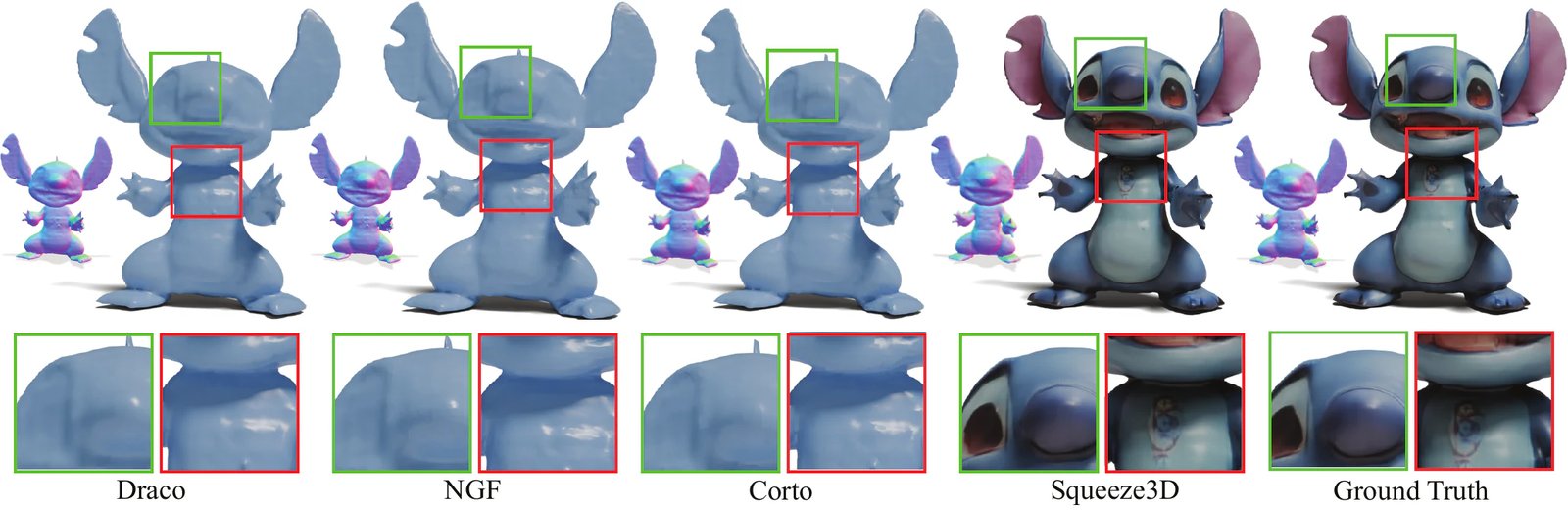
Five renders of a blue cartoon alien character: Draco, NGF and Corto shown as untextured grey-blue geometry, then Squeeze3D and the ground truth fully textured, with zoomed crops of the face and chest. — Mesh comparison from the project page. Draco, NGF and Corto are shown untextured; Squeeze3D's reconstruction comes back with InstantMesh's texture, which flatters it in a side-by-side (Squeeze3D project page, mesh comparison).

Where I'd push back is the comparison. Draco's compressed sizes in Table 2 run from 0.93 to 1.04 MB across quantisation from 4 to 14 bits, which is suspiciously close to the size of one texture image. That would explain why Draco's ratio barely moves (6.20x to 6.92x) however coarsely you quantise: the geometry shrinks and the texture doesn't. Corto, by the paper's own Appendix B.2, is measured "with the texture image stored separately". I can't tell from the paper whether each baseline counts the texture, and the flat Draco curve in Figure 6 looks like a texture floor, not a limit of Draco.

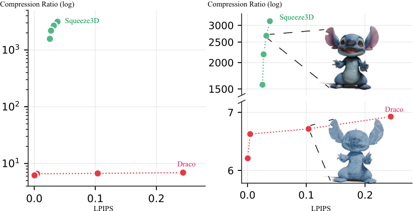
Two scatter plots of compression ratio against LPIPS. Squeeze3D's points sit between about 1,500x and 3,000x with LPIPS near 0.03; Draco's points sit between about 6x and 7x with LPIPS from 0 to 0.24. — Compression ratio against LPIPS for Squeeze3D at several code widths and for Draco at four quantisation settings. Draco's ratio is nearly flat across its whole quality range (Squeeze3D paper, Figure 6).

The fairer comparisons are the learned ones. 3DShape2VecSet, whose pretrained autoencoder the paper also runs as a codec, gets 342.5x at LPIPS 0.1582; DeepSDF gets 131.22x at 0.3704. Squeeze3D's 2,187x at 0.0274 beats both on both axes. Appendix B.1's standardised rate, 0.46 bits per input vertex against 2.86 for 3DShape2VecSet, makes the same point without the file-format question.

Point clouds: 58.5x is mostly ASCII

The point-cloud test files are ASCII PLY. The eight in assets/pc/ each declare 2,048 vertices with three float properties written out as decimal text, 116 to 118 KB each, matching the 117 KB in Table 3. The same 2,048 points as binary float32 take 24,576 bytes. Against that, the 512-number code (2,048 bytes) is a 12x ratio, not 58.5x.

The paper's own standardised rates say the same thing more politely. Table 14 gives Squeeze3D 8.00 bits per point against V-PCC's 9.32, G-PCC's 12.60 and Draco's 20.88 to 29.92. So Squeeze3D uses 14% fewer bits than V-PCC, at a PointSSIM of 0.4484 against V-PCC's 0.9437. On point clouds it is not in the same quality class as the MPEG codecs, and the paper says as much: it "might need further improvements to match the quality of other methods".

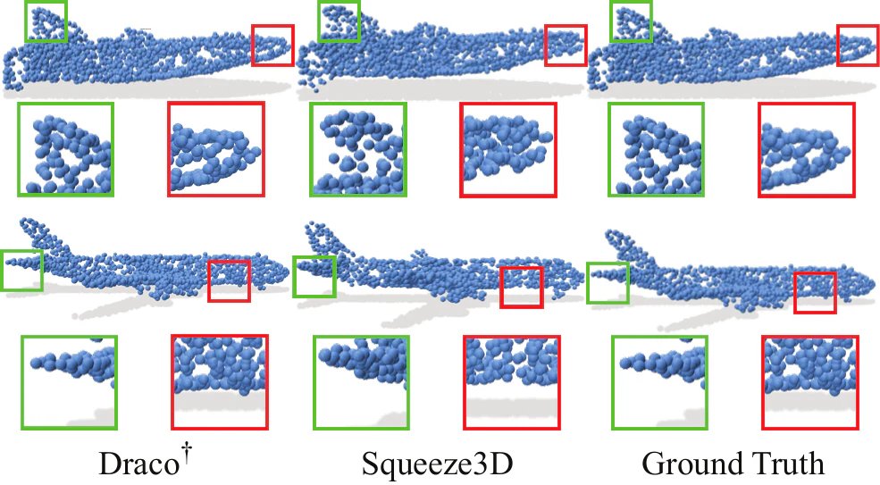
Two airplane point clouds rendered as blue spheres, each shown for Draco, Squeeze3D and the ground truth, with zoomed crops of the tail and fuselage. — Point-cloud reconstructions. The paper notes the Draco column is a much higher-storage operating point than Squeeze3D's (Squeeze3D paper, Figure 7, as shown on the project page).

Two more things about this row. The 512-wide code behind 58.5x has no released checkpoint; the Hugging Face repo ships 1,024, 2,048, 4,096 and 8,192. And PointNet++'s global feature is itself 1,024 numbers, so from 1,024 up the "compressed" code is as wide as the encoder output or wider. For those widths the forward network isn't compressing anything; PointNet++ already did, and the adapter is a translator. The quality numbers are also hard to line up. Table 18 lists the 512-wide model at PCQM 1.4001 and PointSSIM 0.3640 on a separate set of 100 clouds, while Table 3 gives 1.8437 and 0.4484; 1.8437 is the 4,096-wide row of Table 18. Table 3 also gives V-PCC a PCQM of 48.22 when every other entry is between 0.07 and 3.3. I'd treat this table as rough.

Radiance fields: 619x, 634x, or "more than 650x"

The radiance-field code is 24,000 numbers, 96,000 bytes in float32, and Table 11 lists it as 93.75 KB. The original grid averages 58.07 MB. In binary units that is a 634x ratio. Table 4 says 619.41x, which is 58.07 divided by 0.09375, the KB figure read as if it were thousandths of a MB. The abstract says "more than 650x". That comes from Table 16, a separate held-out "ai" subset of NeRF-MAE scenes, which lists 657.89x as 59.21 MB over 0.09 MB, with the code size rounded down to 0.09. On the same denominator as Table 4 that row is 631.6x, and in binary units 646.7x. Under every consistent accounting I can construct, no radiance-field result in the paper reaches 650x. That held-out row is also the weak one: PSNR 22.40 and LPIPS 0.1400, 4.22 dB below the main test set.

The bigger issue is structural. LTNeRFOrtho (lines 657-735) is a U-Net, and the paper's Appendix A.1 says so: skip connections "add encoder feature maps to decoder activations whenever spatial dimensions match". I traced the shapes through the code and checked the channel counts against the released rf_nerfmae.safetensors. Exactly one skip fires: the encoder's output at $20^3$ with 384 channels is added to the decoder at the same resolution (the decoder's layer 8). That tensor is 384 × 8,000 = 3,072,000 numbers, 128 times the 24,000-number code, and it comes straight from the input side. As released, the decompression half cannot run from the code alone. Count the skip tensor and the ratio is about 4.9x. I couldn't run the model, so I can't say how much quality survives if the skip is zeroed; a network trained with it will lean on it.

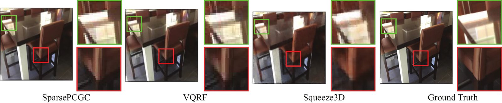
Four renders of a dining table and chair scene from SparsePCGC, VQRF, Squeeze3D and the ground truth, with zoomed crops of a window reflection and a chair leg. — Radiance-field reconstructions against SparsePCGC and VQRF. Squeeze3D's render is softer but holds the structure (Squeeze3D paper, Figure 5, as shown on the project page).

The meshes have a milder version of this. In LTOrtho, fc3 reads ln2(mid + identity), but the example scripts save mid alone (examples/mesh_compression_instantmesh.py, lines 215-218 and 254) and reconstruct from the full forward pass, which still has identity. The saved file can't be decoded on its own. Here the fix costs nothing: store the 770-number sum instead and the ratio is unchanged. The scripts also count the code as float32 throughout. Half precision would double every ratio in the paper, and nobody tested it.

The decoder you have to ship

Following codec convention, the ratios leave out the decoder, and Appendix C.8 does the honest amortisation: a frozen generator plus reverse network of 3.43 GB for InstantMesh breaks even after 534 meshes. My count of the released reverse network alone (ln2 and fc3, 757.9 million float32 parameters) is 2.82 GB, which with InstantMesh's 1.51 GB gives about 4.3 GB and a break-even near 690 meshes. Same order, slightly worse. For an asset library with millions of objects, either number disappears.

What the released weights say

I read the safetensors header of every released checkpoint and summed the tensor shapes. The radiance-field model is 86.46 million parameters, matching Table 9. The other seven are not:

Checkpoint	Table 9 (M)	Released weights (M)
MeshAnything → InstantMesh	96.12	961.16
MeshAnything → OpenLRM	87.51	875.11
MeshAnything → Shap-E	134.53	988.05
PointNet++ → LION, 1,024	2.11	21.13
PointNet++ → LION, 2,048	6.53	65.31
PointNet++ → LION, 4,096	22.29	222.89
PointNet++ → LION, 8,192	81.48	814.87
NeRF-MAE	86.46	86.46

Six of them are off by almost exactly a factor of ten, which looks like a slipped decimal; the README's own "16.6 GB" for the weights is consistent with the larger numbers, not the smaller ones. The InstantMesh file is 3.84 GB. Nearly all of it is fc3, the 983,040 × 770 matrix that writes the triplane, and the counts follow directly from the configs. The Shap-E checkpoint is off by a different factor and has no LayerNorm weights at all, so it was trained with a different class than the LTOrtho its config names. None of this changes a compression ratio, but "small neural networks" undersells a 3.8 GB adapter.

Where it fails

The paper is candid that the generator is a hard ceiling. Squeeze3D cannot reconstruct anything the generator cannot generate, and fine detail outside the generator's prior is "smoothed away or hallucinated rather than reconstructed faithfully". The failure figure shows exactly that: an ornate dragon and the Lucy statue come back plausible and wrong in the small places.

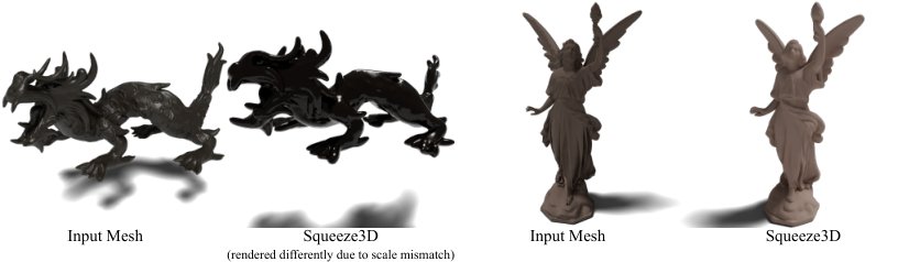
Two pairs of renders: an ornate black dragon and its smoother Squeeze3D reconstruction, and a winged statue with its reconstruction losing fine surface detail. — Failure cases: intricate detail and text are smoothed or invented, because the generator cannot produce them (Squeeze3D paper, Figure 15).

The attribution experiment in Table 21 is the most useful one in the appendix. For both failures, MeshAnything's own decoder reconstructs much better (dragon Chamfer 0.01670) than InstantMesh fed the true views directly (0.15039). The information was in the encoder; the generator couldn't use it. That makes the method only as good as the best open generator, which is the paper's stated upside, since newer generators should slot in by retraining the adapters, and it is also the reason not to use it where geometry must be exact. The broader-impact statement says it plainly: not for safety-critical geometry without a fidelity check and a fallback codec.

Noise robustness is reasonable for meshes at small perturbations (PSNR 27.50 clean, 26.49 at 0.5% of the bounding-box diagonal) and falls off fast after that (20.12 at 2.5%). For anything from a LiDAR scanner, where noise of that order is normal, I'd want to see this on real scans first. The radiance fields degrade more gently, 26.62 to 24.90 PSNR at 10% of the dynamic range.

One question the paper leaves open is reconstruction of the generator's own outputs versus real assets. The adapters train only on generated objects, and the evaluation uses Objaverse, ShapeNet, the ABO scans and NeRF-MAE scenes. The authors flag that the generators may have seen the Objaverse test objects in pre-training, which is why they built a separate set of 500 meshes. Results there are as good as on the main test set (LPIPS 0.0124), so the out-of-distribution story holds for meshes.

What I'd take from it

The method is worth knowing for the bridge, not the codec. Two frozen models, paired data made by running one of them forward, an MSE in the target's latent space and a redundancy term on the code: that recipe should work for any pair of models where you can sample one side, and the Gram loss is cheap and has the clean interpretation above. If I were bridging, say, a point-cloud encoder into a newer generator, this is where I'd start, and I'd store the code in fp16 on day one.

As a codec, it is a good fit for archives of textured assets that resemble what the generator already makes, where a 3 KB code and a shared 4 GB decoder are a fine trade and "looks right" is the spec. For point clouds it trades a lot of quality for a small rate gain over V-PCC. For radiance fields, the released network isn't a bottleneck yet, and I'd want to see the skip removed and retrained before quoting any ratio.

If you work with splats rather than these formats, the site's pieces on the SOG splat format and on compressing Gaussian colour cover the conventional end of the same problem. On the regulariser side, LeVJEPA and H-JEPA use SIGReg, the distributional cousin the thread also cites, to keep embeddings from collapsing, and the Muon piece covers the optimizer most of these adapters were trained with.

How I checked

I read v2 of the paper (the TMLR version, 28 September 2026) from arXiv's HTML, including all appendix tables, and cross-checked every ratio by dividing the paper's own sizes in binary and decimal units. I shallow-cloned the repository at commit e6c950c (25 September 2026), read the mapping networks, training loop, configs and example scripts, and quoted them with line numbers from that commit. I counted vertices and file sizes on the repo's sample point clouds and meshes. For the weights, I fetched only the safetensors headers of all eight files on Hugging Face with HTTP range requests and summed the tensor shapes; nothing was downloaded beyond the headers and nothing from the repository was executed. The skip-connection trace is by hand, from the layer definitions, checked against the released tensor shapes. The toy in the first widget is my own code (components/articles/squeeze3d/gram-toy.ts), deterministic, and only illustrates the loss; its numbers are not the paper's. I could not run any of the models, so the quality numbers are all the paper's, and I could not test how the radiance-field model behaves without its skip connection.