2026-10-06 · 20 min · world-models · self-supervised-learning · representation-learning · pde · robotics · explainer
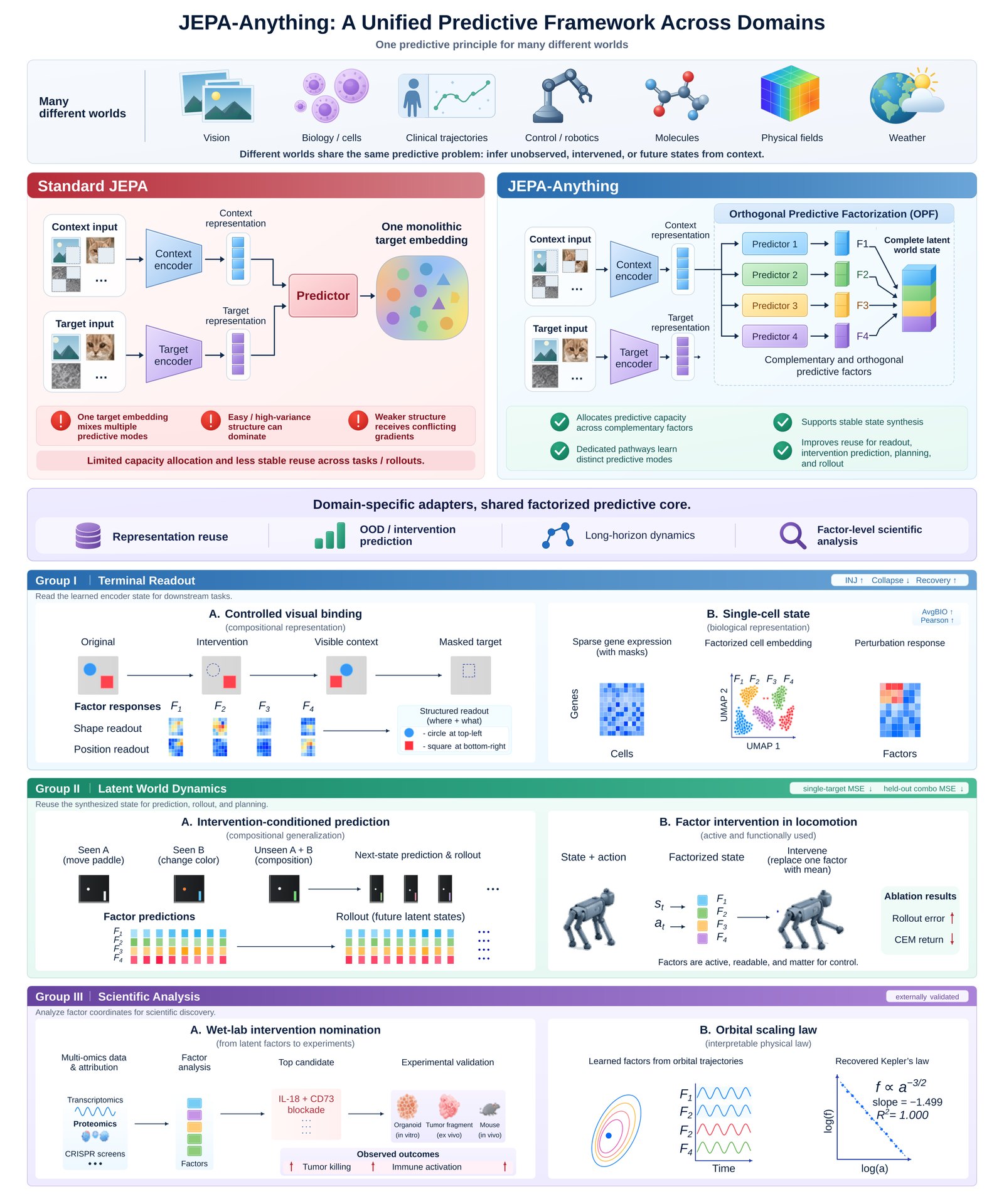
The launch post for JEPA-Anything says "one world model that works across molecules, cells, fluids, patients, robots, or even weather." The paper (arXiv 2609.20800, from PhAI Labs, CUHK and others, code at Gen-Verse/JEPA-Anything) is more careful than the post. Its own README says it in one line: "domains need not share a single encoder or one set of model weights."
So the first thing to get right is what is shared. It is a training recipe and a latent interface, not a network. I counted the released weights on the Hugging Face dataset: 36 checkpoint files, one or more per task, from 1.9 MB to 419.2 MB, about 0.91 GB in all (measured, from the Hub API). A weather checkpoint cannot read a molecule.
That is not a criticism of the idea, which is a small change to how a JEPA predicts that bolts onto any existing JEPA. This piece explains it from the ground up, then checks the numbers.
- license
- Apache-2.0
- branch
- main
- tests
- 8 files
- source
- 264.3 kB
- commit date
- 2026-09-18
by size of tracked source at this commit, file counts in brackets; docs, data and vendored trees excluded
local clone, 2026-10-06 at c6e6c88 — branch, commit, commitDate, fileCount, hasTests, languages, license, licenseFile, shallow, testFileCount
shallow clone: counts describe the pinned tree, not the history
A JEPA in four parts
A joint-embedding predictive architecture learns by predicting one part of the world from another, in representation space rather than in raw observation space. It has four moving parts:
- A context encoder reads what is visible (unmasked patches, the past, the current state) and produces .
- A target encoder reads the thing to be predicted and produces .
- A predictor maps , plus a descriptor of which target is wanted (a patch position, a time step, an action), to a guess .
- A loss pulls toward .
Why predict in latent space? Because a pixel loss pays for every pixel. Predict the next frame of a pond and most of the loss is in the ripples, which are unpredictable and useless. A latent target lets the target encoder decide what level of detail is worth predicting.
The catch is collapse. If the target encoder and the predictor are both learned, the loss has a trivial minimum: map everything to the same vector. The common defences:
- EMA target and stop-gradient (I-JEPA, V-JEPA): the target encoder is an exponential moving average of the context encoder and gets no gradient, so it cannot chase the predictor.
- Variance and covariance regularisers (VICReg): penalise any embedding coordinate whose standard deviation across the batch falls below a floor, and penalise correlated coordinates.
- Distributional regularisers (SIGReg in LeVJEPA): push the embedding distribution toward an isotropic Gaussian and drop the EMA branch entirely.
JEPA-Anything uses the first and borrows the spirit of the second. The target encoder is an EMA, , with a stop-gradient on its output. On top of that it adds two hinge-style variance floors, described below. SiamJEPA and NextLat are two other recent takes on the same family, if you want a comparison of collapse machinery.
The problem OPF is aimed at
A standard JEPA predicts its target with one predictor and one target vector. The paper's argument is that a real target mixes several predictive modes: a future patient state carries the risks of hundreds of events, a physical field has slow and fast modes. Squeezed into one regression target, the easy or high-variance part dominates the gradient, several latent directions do the same job, and the weaker structure gets conflicting updates.
Their fix is to make the predictor's capacity allocation explicit. They call it orthogonal predictive factorization (OPF).
How OPF works
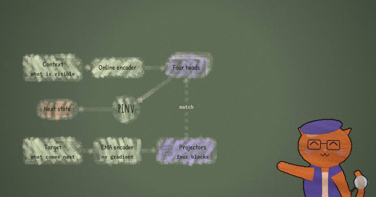
Take a latent target from the EMA encoder and stop its gradient. Learn projector matrices with , so together they form a square matrix . Each projector reads off one block of coordinates:
Each block gets its own predictor , which sees the same context representation and the same target descriptor: . The prediction loss is a plain mean squared error per block. It regresses magnitude as well as direction, because the blocks have to be put back together later:
Nothing so far stops all projectors from learning the same directions. That is the job of the orthogonality loss, which asks each projector's columns to be orthonormal and different projectors to be orthogonal to each other:
The two activity terms are hinge penalties on standard deviations, measured across the mini-batch. penalises any projected target coordinate whose standard deviation drops below ; it shapes the projectors, since the target itself is stopped. does the same for every coordinate of the online context representation, which sends a direct anti-collapse gradient into the encoder. Each domain keeps whatever loss its original implementation already had and adds the OPF terms:
The paper's appendix gives
for every dynamics task and 0.02, 0.10, 0.02 for the three locomotion tasks (reported, Table 10). The
released library's jepa_anything_objective() defaults all three weights to 1.0 and both floors to
0.1 (measured, losses.py), so if you use it, set them yourself.
Putting the state back together
The predicted blocks are concatenated into and turned back into one state with the Moore-Penrose pseudoinverse of the analysis map:
When is exactly orthogonal, and this is just : add up each block's contribution. The paper's Corollary 1 is the reason orthogonality matters here. If the factor predictions are off by an error , the state is off by , whose size is at most . An orthogonal has every singular value equal to 1, so the state error equals the factor error. A with two nearly parallel columns has a tiny , and a small factor error becomes a large state error.
The widget below is that argument in two dimensions: two projector directions, a fixed true state , and a factor error that pushes one coordinate up and the other down. Close the angle and watch the pseudoinverse estimate fly off while the condition number climbs.
The error vector pushes factor 1 up and factor 2 down by the same amount. At 90° both syntheses land on the same point and the state error equals ‖e‖. Close the angle and the pseudoinverse still recovers z exactly when e = 0, but every unit of factor error becomes up to 1/σ_min units of state error; transpose synthesis is wrong even with perfect factors. Preset: the zero-penalty limit of Proposition 1; the toy matches its condition number only. In two dimensions a κ of 438.52 is an angle of about a quarter of a degree.
In words: at 90 degrees is 1 and a factor error of 0.10 is a state error of 0.10. Shrink the angle and the worst-case amplification grows without bound. Transpose synthesis, just summing the blocks, is wrong even with perfect factors once the projectors stop being orthogonal, which is why the paper uses the pseudoinverse.
Where actions and interventions go
For a world model, the next state depends on something the agent or experimenter does: an action, an intervention label, a known forcing. The paper calls it and lets the domain adapter put it either into the context tokens or into the target descriptor. A transition is then
and applying it repeatedly gives a latent rollout. A planner scores rollouts with the domain's own reward. In the locomotion experiments that planner is CEM: sample many action sequences, roll each forward through the model, keep the first action of the best one.
After training, representation mode discards the EMA encoder, projectors and heads and puts a readout on the online encoder; operational mode keeps them and feeds the synthesised state to a decoder, a planner or the next rollout step.
One interface, many adapters
Here is where "Anything" comes from. Each domain writes an adapter that turns a raw observation into content tokens and structural descriptors (a patch coordinate, a time stamp, a graph position, or nothing), and a view sampler that chooses which tokens are context and which are target. Everything after that follows the one algorithm. The paper's Table 1 is explicit about the boundary: raw representation, tokenisation, context-target semantics, encoder architecture (ViT, Transformer, GNN, MLP) and the readout are domain-specific. The EMA scheme, the factorised predictors, the regularisers and the additive loss are shared.
released weights, measured: Shapes3D checkpoints, a 192-wide ViT on 64×64 images, 13.4 MB: not the Table 3 backbones
Pick a domain. Everything drawn in purple changes: the input, the adapter that turns it into tokens, the encoder family, the readout. The green block is drawn the same every time because it is the paper’s actual claim: an EMA target, K projectors, K small predictors and a pseudoinverse that stitches their outputs back into one state. Only its widths change. Every domain trains its own weights.
The table that matters, condensed from the paper's Table 2:
| Domain | Context → target | Backbone | |
|---|---|---|---|
| Vision (MuJoCo scenes) | visible patches → masked patch states | DINOv3 ViT-S, SigLIP2 Base | 384; 4×96 and 768; 4×192 |
| Single cell (kidney, PBMC-10K, Adamson, Norman) | masked expression → complete cell state | scGPT | 512; 4×128 (Norman) |
| Clinical (UK Biobank cohort) | patient history → future patient state | GPT-2 small | 768; 4×192 |
| Interventions (CITRIS Pong) | observation + intervention → next state | matched encoder and predictor | 160; 5×32 |
| Dynamics (CausalWorld, DMC, PDEBench, WeatherBench2) | state, frames, action or forcing → next state or field | matched task-specific | 128; 4×32 |
| Locomotion (Hopper, Walker2d, HalfCheetah) | state + action → future state | latent dynamics + CEM | 32; 4×8 |
| Molecules (water, quartz, paracetamol, benzene) | atomic state → future state | TrajCast-style -equivariant | 64; 4×16 channels |
The molecular case is the neatest adaptation. An equivariant network carries vector features as irreps with three components each, and a projector that mixed those components would break rotation equivariance. So OPF acts only on the 64-channel multiplicity axis, as : the same channel projection applied identically to x, y and z.
What is in the released weights
I did not run the authors' code. I read the checkpoint pickles with a restricted unpickler that never imports a class, and the projector tensors as raw float32 arrays.
The dynamics checkpoints are small multilayer perceptrons. The CausalWorld model is an encoder from a 56-number state through two 256-wide layers to , an identical EMA teacher, a shared trunk whose first layer reads 137 numbers (the 128-wide latent plus a 9-number action), four 128 → 32 heads, a decoder, and a projector tensor of shape (4, 128, 32). That is 393,400 online parameters (measured). The WeatherBench2 model has the same layout with a 6,144-number flattened field as input: 3,514,496 online parameters, a 20.8 MB file (measured). That is the paper's "shared trunk followed by branch-specific heads" option, and it is a long way from a weather model in the GraphCast sense. The paper compares it only with a matched monolithic JEPA, never with a weather-specific forecaster.
The projectors are where it gets interesting. The paper's mechanism audit (Table 5) reports, on CITRIS Pong, a cross-factor overlap of , and for orthogonal factorization, against an overlap of 0.4550 and for unconstrained multi-head prediction (reported). An overlap at the level of float rounding error is what an exactly orthonormalised basis gives, and the paper does say that "the controlled geometry analysis uses this strict decomposition", a QR factorisation. The predictive models instead use soft-regularised projectors and pseudoinverse synthesis. So I measured those:
| Released checkpoint | worst-case error amplification | ||
|---|---|---|---|
| HalfCheetah, 20-step | 1.0000 | 1.000 | 1.0x |
| CausalWorld pushing | 0.9312 | 1.140 | 1.07x |
| CITRIS six-step, five seeds | 0.6742 – 0.7280 | 1.683 – 1.819 | 1.37 – 1.48x |
| PDEBench shallow water | 0.4788 | 3.988 | 2.1x |
| PDEBench Burgers | 0.2596 | 6.679 | 3.9x |
| APEBench Burgers | 0.2764 | 7.969 | 3.6x |
| WeatherBench2 | 0.1784 | 9.175 | 5.6x |
| Synthetic PDE | 0.0218 | 63.287 | 46x |
| CITRIS legacy (three-channel protocol) | 0.0082 | 227.491 | 122x |
Singular values and condition numbers are measured; the amplification column is reasoned, from the
paper's own bound. The locomotion projector is orthogonal to float precision, which suggests it was
retracted with QR (the library has a qr_retraction mode). CausalWorld is close behind; the rest drift further. Five of the nine have a
condition number above 6, and the Synthetic PDE projector is closer to the paper's "unconstrained
heads" than to its "orthogonal factorization" column. The CITRIS legacy checkpoint is labelled on its
card as an earlier protocol, so it is not evidence against the paper, but it is in the release.
Two honest readings. One: the soft penalty with is too weak to hold these projectors near orthogonal, and Table 5 describes the idealised geometry rather than the trained models. Two: the method still beats the matched JEPA on Burgers and WeatherBench2 with near 7 to 9, so whatever is doing the work there is not exact orthogonality. More heads, the variance floors and the per-block loss are all candidates. The paper does not separate them, apart from the CITRIS audit against an unconstrained multi-head baseline, and that audit reports geometry, not prediction error.
Results, against the matched JEPA
Every quantitative comparison holds the adapter, encoder, sampler, budget, split and readout fixed and swaps the monolithic JEPA term for the OPF terms. That is a clean ablation, and it is the right experiment for the paper's claim. It is not a comparison against the best model in each field, and the post's "works across" should be read with that in mind.
Terminal readout: vision, cells, patients
- Vision binding (Table 3, reported). On DINOv3, held-out-cell accuracy goes .572 → .581 and collapse rate .426 → .417 against standard JEPA; the frozen checkpoint with the same learned-grid readout already scores .569. On SigLIP2 it is .483 → .490. About one point, over ten seeds, no spread reported.
- Single cell (Table 4, reported). PBMC zero-shot AvgBIO is 0.5288 for scGPT, 0.7194 for Cell-JEPA and 0.7752 for JEPA-Anything; Norman perturbation Pearson is 0.631, 0.787 and 0.814. Most of the jump comes from going latent at all (scGPT to Cell-JEPA); OPF adds a smaller but consistent step on top.
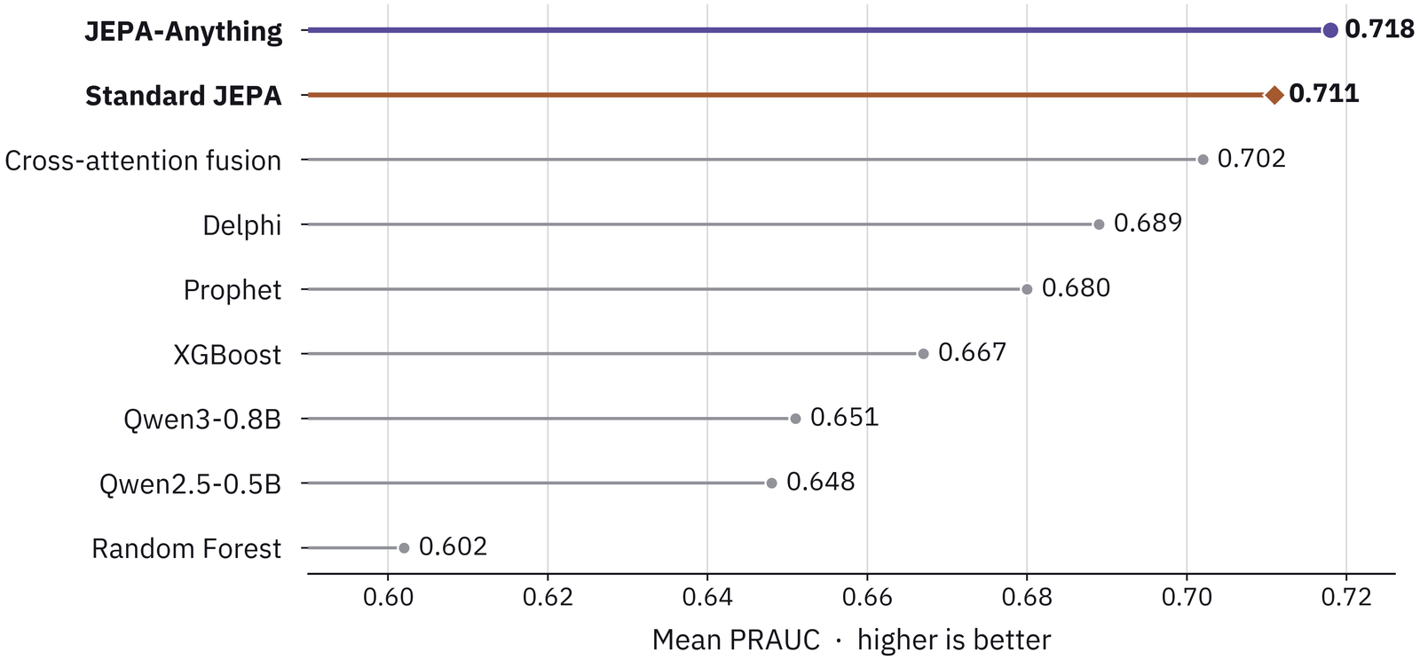
- Clinical (Figure 3, reported). Mean PRAUC over more than 1,000 future events is 0.718 against 0.711 for the matched JEPA, with a cross-attention fusion model at 0.702, Delphi at 0.689 and XGBoost at 0.667. The 0.007 gap (reasoned) is real money in a clinical ranking but small next to the spread between methods; no seed variance is shown.
Interventions and dynamics
On CITRIS Interventional Pong the model sees a frame plus a label of which game variables were externally changed, and predicts the next frame. Single-intervention one-step MSE falls from 0.009541 to 0.006218, combined interventions (a combination withheld in training) from 0.009441 to 0.008223, and six-step free rollout from 0.009478 to 0.008665: reductions of 34.83%, 12.90% and 8.58% (reported).
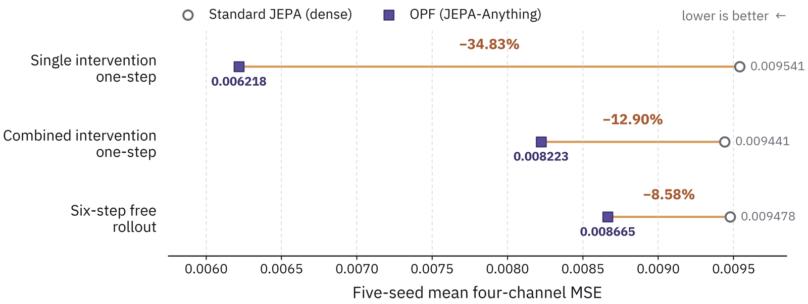
The released CITRIS weights are the five-seed models trained with six-step feedback. Their card reports one-step MSE of 0.00952107 against 0.00682598 for single interventions, which is a 28.3% reduction (reasoned), and 0.00942106 against 0.00822350 for combinations. The paper's 34.8% comes from a training condition whose weights are not released.
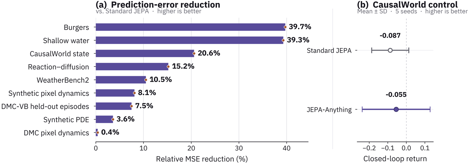
The ten-task dynamics benchmark is the broadest evidence. Relative MSE reduction against the matched JEPA ranges from 39.7% on PDEBench Burgers and 39.3% on shallow water down to 3.6% on a synthetic PDE and 0.4% on DMC pixel dynamics (reported, Figure 5). The tenth task is CausalWorld closed-loop control, where the mean return is −0.055 against −0.087: both negative, with error bars that overlap almost entirely. The abstract's "improves reported metrics on all 10 dynamics tasks" is true of the means.
The rollout table shows the errors do not compound faster: on PDEBench Burgers, MSE goes 0.001830 → 0.006369 from step 1 to step 6 for the JEPA and 0.001101 → 0.004014 for JEPA-Anything (reported, Table 6). On the APEBench protocol, Burgers held-out late-state error drops by about 49.5% and six-step rollout by 44.7%, and Kuramoto–Sivashinsky by 13.2%, in every seed (reported). The capacity-matched 50-step Burgers test is the sobering one: the gain is −5.84% at 20 steps and −3.15% at 50, narrowing as the horizon grows.
The Hugging Face folder for this benchmark holds 15 task checkpoints, including CLEVRER, Navier-Stokes and a 2-D reaction-diffusion run that the paper does not report (measured). The paper does not say whether those were evaluated.
Planning and locomotion
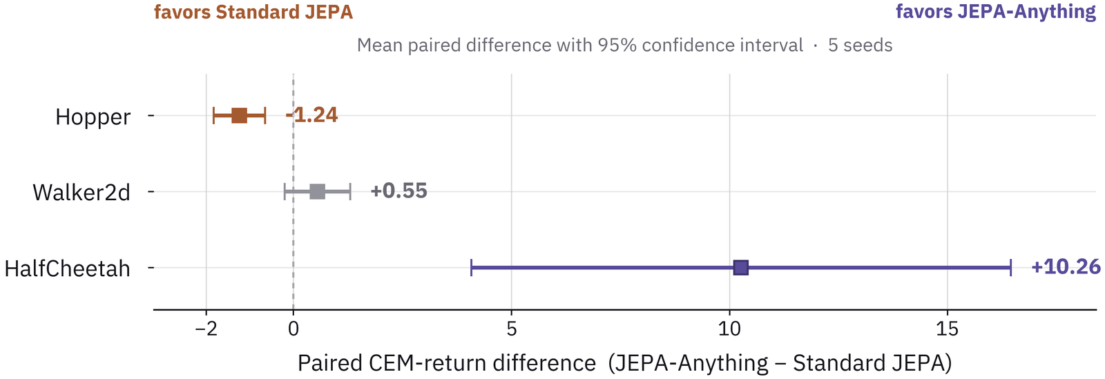
This is the one place the paper reports a loss. Paired CEM return favours standard JEPA on Hopper (−1.24), is +0.55 on Walker2d with a confidence interval that crosses zero, and +10.26 on HalfCheetah (reported, Figure 6). The authors say it plainly: planning performance is environment-dependent.
The factor ablation is better evidence that the four blocks are each doing something. Replacing any one factor by its training-set mean raises 20-step rollout error in all three environments, and on HalfCheetah masking F1 or F3 lowers return in all five seeds (reported). The single-factor probes find each block linearly predicts a different body variable best on Hopper, with between 0.294 and 0.424: modest, and the paper is careful to call them "motion preferences" rather than labels.
Molecules
With a TrajCast-style equivariant forecaster, JEPA-Anything has the lowest one-step displacement MAE and 100-step RMSD on all four systems (reported, Table 9). Paracetamol 100-step RMSD is 3.155 Å from scratch, 1.868 Å with JEPA pretraining and 1.776 Å with OPF. Water goes 2.536 → 2.459 Å. As elsewhere, the big step is from scratch to any JEPA; OPF is a smaller step on top. The released molecular checkpoint is a 3.1 MB TiTo/PaiNN model with a latent flow-matching module (measured, from its file list and card), not the TrajCast-style setup in the table.
The science claims
Group III is where the paper reaches furthest, and where I can check least.
The cancer case says factor analysis "nominated IL-18 combined with NT5E/CD73 blockade", and wet-lab studies in co-culture, patient-derived organoids, tumour fragments and mice supported it. The paper gives one figure of selected organoid and fragment results and no protocol, no list of other candidates the factors ranked, and no description of the "domain-specific intervention analysis" that turned factor coordinates into a drug pair. I cannot evaluate it from what is published.
The orbital case is checkable in principle. From simulated position-velocity trajectories, spectral analysis of the latent factor coordinates finds frequencies that scale with semimajor axis as , with a fitted slope of −1.4991 and (reported).
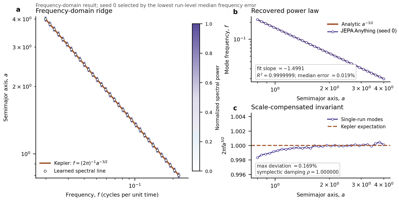
Two things temper it. The figure's own header says the run shown was "selected by the lowest run-level median frequency error", so it is the best seed, not a typical one. And the simulated orbits obey Kepler's law by construction, so a model that predicts them well must carry each orbit's period somewhere in its state (reasoned). What the result shows is that OPF's factor coordinates expose that period cleanly enough for a spectral fit. That is a useful property of the coordinates. It is not the model discovering a law it was not shown.
What the repository is
The GitHub repo is a library, not a training codebase. jepa-anything-core has 2,069 lines of Python
across five modules: the projection and pseudoinverse synthesis, the four loss terms, matched
baselines with parameter and FLOP accounting, and geometry audits (measured). A
jepa-anything-skill folder holds a design validator and a scaffold generator meant to be driven by
a coding agent, and one synthetic recipe that checks interfaces. Its README is direct about it: the
example "does not train a model or produce benchmark performance", and the checkpoint manifest
records an untrained example with no performance claims. The domain training code is not there. The
per-task model code and checkpoints are on the Hugging Face dataset, Apache-2.0, alongside inference
scripts.
Two more mismatches between paper and release. The vision checkpoints are a 192-wide ViT on 64×64 Shapes3D images, 13.4 MB, not the DINOv3 ViT-S and SigLIP2 backbones in Table 3 (measured). And the clinical model has no checkpoint at all; its row on the dataset card reads "progressive checkpoint release".
What to take from it
Strip away the "world model everything" framing and JEPA-Anything is a clean, portable change to the predictor of any JEPA: split the target into blocks with learned, softly orthogonal projectors; give each block its own small head; keep every coordinate alive with variance floors; stitch the blocks back together with a pseudoinverse so the full state survives for rollouts and planning. It costs almost nothing. The locomotion models differ from their dense baselines by under 0.3% in parameters and 2% in prediction-head FLOPs (reported).
The evidence that it helps is broad and mostly shallow. It beats a matched monolithic JEPA in nearly every comparison, sometimes by 40%, often by a point or less, and once it loses. It is never compared with the strongest specialist model in a field. The geometry that justifies the design is exact in the paper's audit and approximate, sometimes loose, in the shipped weights. If you already run a JEPA for dynamics or rollouts, OPF is a cheap ablation to try. If you read the launch post as one network that forecasts weather and molecules, that is not what the paper built, and the paper says so.
For a different direction on the same family, LeVJEPA removes the EMA target altogether, and Cosmos 3 is what a world model looks like when it is built as one large generative network rather than as a recipe.