2026-10-06 · 26 min · world-models · self-supervised-learning · representation-learning · robotics · reinforcement-learning
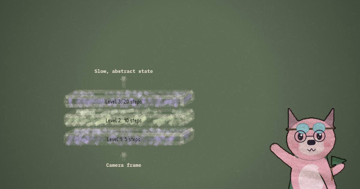
Why read this
Hightop 30%How H-JEPA's levels, SIGReg and top-down planner work, with the two gains split apart, and where the paper's own tables and code disagree.
- Interactive explanations
- Original analysis
- Runs on a consumer GPU
Robotics & embodiedMITResearch paper
How this was scored
- Is it new?
- 2 of 3: A real new idea, method or capability
- Can I trust it?
- 2 of 3: Measures key facts from files, code or configs
- Can I run it?
- 2 of 3: Open code or weights with real limits
- Will I understand it?
- 3 of 3: Mechanism carried by interactives built from real code or data
- Can I act on it?
- 2 of 3: A concrete recipe, numbers or comparison
- Will it last?
- 2 of 3: A reference for a year or more
- Does it affect many?
- 1 of 3: A specialist community
- Only here?
- 2 of 3: A teardown or measurement few others did
Score 71 of 100, ranked 90 of 445 rated articles. Each question is answered 0–3 by hand, and a 3 is rare. How articles are scored
Randall Balestriero's announcement calls H-JEPA "the first end-to-end learned hierarchical world model for long-horizon visual planning." I clicked because of the second post in his thread: "Semantic abstraction yields temporal compression!" It is a strong claim about where hierarchy comes from. It says nobody has to design the levels. Ask each level to predict farther ahead, and the level throws away whatever it cannot predict at that distance, and what is left is slow and abstract on its own.
The paper is arXiv 2610.06805, by Wancong Zhang, Basile Terver, Michael Rabbat, Yann LeCun and Balestriero, with code at kevinghst/H-JEPA under MIT and 93 checkpoints on Hugging Face. I read all three. The headline number holds up: on Visual AntMaze, a three-level model raises planning success from 18% to 73%. What I did not expect is how carefully the paper takes that number apart. It isolates two different reasons hierarchy helps, shows one of them working with no hierarchical planner at all, and admits two environments where neither shows up. Then an appendix proves that the regularizer the whole recipe rests on is blind to a specific failure on real robot video. I found that appendix more useful than the headline.
- license
- MIT
- branch
- main
- tests
- none found
- source
- 721.1 kB
- commit date
- 2026-10-06
by size of tracked source at this commit, file counts in brackets; docs, data and vendored trees excluded
local clone, 2026-10-06 at 840e76b — branch, commit, commitDate, fileCount, hasTests, languages, license, licenseFile, shallow
shallow clone: counts describe the pinned tree, not the history
A world model that never draws a pixel
H-JEPA builds on LeWorldModel, or LeWM, from the same group, so start there. A JEPA world model has three parts. An encoder turns an image into a vector . An action encoder turns the command into a vector. A predictor takes the current latent and the action and guesses the next latent. Training minimises the squared error between and the encoder's own . No decoder, no reward, no pixels in the loss. If you have read the site's piece on next-latent prediction, it is the same idea with actions in the loop.
Planning with it is pleasantly direct. Encode the current frame and a goal frame. Start from a batch of random action sequences, roll each through the predictor, measure how far the last predicted latent lands from the goal latent, and push the actions downhill on that distance with gradient descent. Execute the first couple of actions, look again, repeat. Model predictive control, with a learned model doing the predicting.
The catch is the one every JEPA has. The easiest way to predict your own next latent perfectly is to make every latent the same. A constant encoder gets zero prediction loss and encodes nothing. Earlier JEPAs stopped this with an EMA teacher, a stop-gradient, VICReg-style variance and covariance terms, or a frozen pretrained encoder. LeWM's claim was that you need none of that: two loss terms, prediction plus SIGReg, trained from pixels end to end. H-JEPA's whole recipe depends on that being true at every level of a stack, so SIGReg deserves a proper look.
SIGReg, from the formula to the 35 lines that ship
SIGReg comes from Balestriero and LeCun's LeJEPA, which the site covered through its video descendant LeVJEPA. The target is an isotropic Gaussian: embeddings should look like draws from . Testing that in dimensions directly is hopeless, so it leans on the Cramér-Wold theorem: a distribution is Gaussian if and only if every one-dimensional projection of it is. Pick random unit directions , project the batch to , and run a one-dimensional normality test on each:
is the empirical characteristic function of the projected values, is the standard Gaussian's characteristic function, and the outer weights low frequencies. This is the Epps-Pulley statistic. Each level of H-JEPA adds it to its prediction loss with a weight :
The released implementation is short enough to read whole. Its core is
h_jepa/loss.py:16-47:
def __init__(self, knots=17, num_proj=1024):
    t = torch.linspace(0, 3, knots, dtype=torch.float32)
    dt = 3 / (knots - 1)
    weights = torch.full((knots,), 2 * dt, dtype=torch.float32)
    weights[[0, -1]] = dt
    window = torch.exp(-t.square() / 2.0)
    ...
def forward(self, proj):            # proj: (T, B, D)
    A = torch.randn(proj.size(-1), self.num_proj, device=proj.device)
    A = A.div_(A.norm(p=2, dim=0))
    x_t = (proj @ A).unsqueeze(-1) * self.t
    cos, sin = x_t.cos().mean(-3), x_t.sin().mean(-3)
    ...                             # all_reduce of cos/sin across ranks
    err = (cos - self.phi).square() + sin.square()
    statistic = (err @ self.weights) * n
    return statistic.mean()
Three details are worth knowing. The integral is a trapezoid rule on with 17 knots,
doubled because the integrand is even, so the interior weights are 2 * dt and the ends dt.
The directions are redrawn every call, 1,024 of them, so over training the test covers far more
than 1,024 directions. And the mean over samples is taken over the batch axis of a
(T, B, D) tensor: one normality test per timestep, across the sequences in the batch.
Hold on to that last point. It matters a lot on DROID.
The appendix adds one engineering fix I liked. The statistic is a property of the whole batch, so computing it per GPU and averaging gives a different number depending on how many GPUs you use. The authors all-reduce the real and imaginary ECF before the quadrature instead, two tensors per call whatever the batch size, and show in their Table 11 that the result becomes exactly invariant to sharding, where LeWM's single-GPU version drifts by 14% between one shard and two. If you train SIGReg models across devices, copy that.
The widget below runs the same arithmetic on a toy batch of 256 embeddings in two dimensions, sweeping 16 directions instead of 1,024 random ones. Try "dimensional collapse": one axis survives, so projections along it pass, and only the directions near the dead axis fail. That is why one direction is never enough. Then try "slow-feature collapse", which I explain further down.
An isotropic Gaussian cloud. Every direction passes; the average sits at the statistic's noise floor, near 1 in expectation, which is where the paper says a healthy run settles.
The paper's training curves give a scale for these values. A healthy run's statistic drops fast early in training and settles "within a small factor of its value on exactly Gaussian embeddings, about 1." On collapsed data it grows linearly with the batch size , which keeps the anti-collapse gradient per sample constant.
Stacking the JEPAs
H-JEPA is a stack of these world models where each level reads the level below instead of
pixels. Level 1 is exactly LeWM: a ViT-Tiny over the image, its [CLS] token through an MLP
projector, and a four-layer causal transformer predictor with adaptive LayerNorm action
conditioning. Every level above it has its own encoder, its own action encoder and its own
predictor, and two temporal knobs. The stride says how many lower steps one upper step
covers. The window says how many lower states one upper state summarises:
Every experiment in the paper uses and in simulation, so the upper state encoder is a two-layer MLP applied to every other lower latent, and the action encoder, a one-layer transformer, pools the two lower action embeddings in between into a 4-dimensional macro-action. A level-1 step already spans 5 environment steps, so level 2 predicts 10 steps at a time, level 3 predicts 20, and level 4 predicts 40.
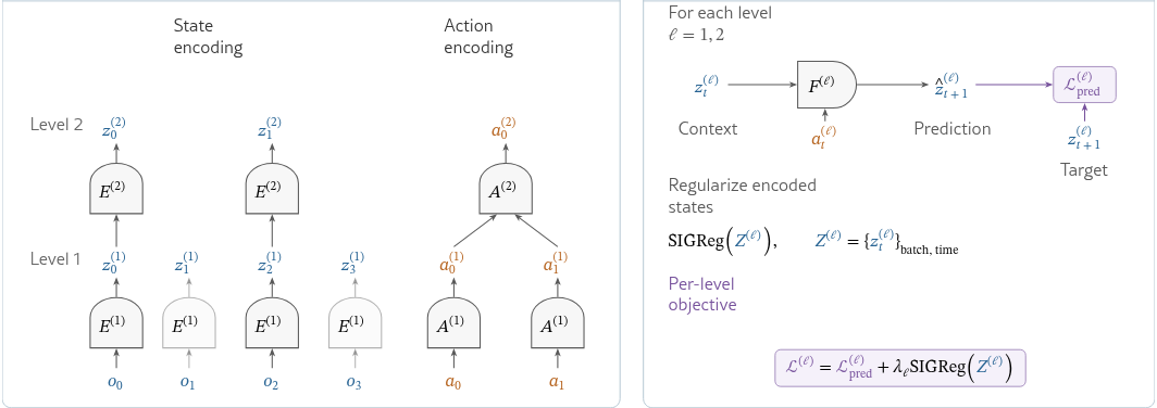
The part that makes this "end to end" is simple to state and the reason the paper exists. All
levels train together from scratch, and the upper levels' losses backpropagate into the lower
encoders. The code just sums the per-level losses, h_jepa/hjepa_utils.py:172:
total_loss = level_loss if total_loss is None else total_loss + level_lossThere is no detach between levels and no stop-gradient on targets. So the level-1 encoder is shaped by every level above it, and every level's latent space is free to collapse under its own predictor. The obvious hack would be to train level 1, freeze it, train level 2 on top. The paper has that variant, calls it stagewise, and uses it only for analysis. Joint training is only safe because SIGReg holds every level's latents open at the same time, with the same weight per level: 0.18 on FourRoom and 0.09 everywhere else. The four-level training curves in the appendix show no level's prediction loss sliding toward zero, which is what a collapse looks like.
- task
- robotics
- library
- pytorch
- license
- mit
- largest file
- 348.2 MB
- files
- 188
- downloads
- 0
- likes
- 0
repo last modified 2026-10-06
One thing surprised me in the released files. The upper levels are not small. On AntMaze the flat LeWM checkpoint is 49.6 MB, and each extra level adds about 45 MB: 94.6 MB for two levels, 139.5 MB for three, 184.5 MB for four. The level-2 predictor is a five-layer transformer with 12 heads, which costs as much as the whole level-1 model. A three-level H-JEPA is roughly three LeWMs glued together, which is worth knowing before you call it cheap. The planner is a different story; I come back to it.
What the upper levels throw away
Thread post two claims abstraction emerges. The evidence is a probing experiment. Freeze a trained four-level model, fit a small MLP probe on each level's latents to recover a physical quantity, and report the error normalised by the quantity's variance, so 0 means perfect and 1 means no better than guessing the mean.
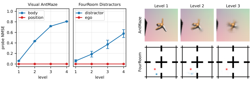
On AntMaze, the ant's 27-dimensional body state becomes steadily harder to read from levels 2, 3 and 4, while its global position stays near-perfectly recoverable. On FourRoomDistractors, the distractor dot fades and the agent stays. The paper's explanation is the one from the thread, and I find it convincing because it is mechanical rather than mystical. The encoder at level only gets gradient from a predictor asked to look environment steps ahead. The ant's joints oscillate many times between two level-3 states 20 steps apart, so encoding them only adds prediction error; the position drifts slowly and stays predictable. The FourRoom distractor teleports at Poisson intervals with a mean of 35 steps, and a longer horizon is more likely to straddle a teleport.
The paper is honest that this is conditional. Figure 5 relates the effect to a "frequency gap", the ratio of the spectral centroids of the fastest and slowest state components. Humanoid, AntMaze and FourRoom have gaps of 3.1 to 12.7 times and show the effect. Push-T, OGBench Cube and DROID have gaps of 1.2 to 1.6 times and show little of it: in a pushing task, the block and the pusher move on the same timescale, so there is nothing slow to keep and nothing fast to drop. So "semantic abstraction yields temporal compression" is true when the world has separated timescales, and that condition decides almost everything that follows.
Planning from the top down
Planning starts by encoding the current frame and the goal frame at every level. The top level then optimises macro-actions so that its last predicted latent lands on the goal:
Each level below plans primitive or less-macro actions, but it is not scored in its own space. Its predicted rollout is lifted through the upper encoder, , and compared with the subgoals the level above predicted:
with the number of subgoals matched. In the closed-loop simulation runs : each level only has to reach the first state the level above imagined. Level 1's actions are executed for two blocks, 10 environment steps, and then the whole stack replans from the new frame.
I went in expecting CEM or MPPI, the sampling planners most latent world models use. The
optimiser is gradient descent through the rollout at every level: AdamW, at most 90 iterations,
early stopping when the best cost stalls, keep the lowest-cost candidate. Macro-actions have no
natural bounds, so the code keeps the last 4,000 macro-actions seen in training, initialises
candidates from a Gaussian fitted to them, and clips them after every step to that queue's 2nd
and 98th percentiles (stable_worldmodel/solver/gd.py:193-194). Without that, gradient descent
would happily wander into macro-actions the upper predictor has never seen. The top-down loop
itself is plain, h_jepa/hierarchical_solver.py:121-213, trimmed:
for level in range(len(self.level_models), 0, -1):
    if level > 1 and planning_horizon == 1:
        continue                     # a one-step upper plan yields no useful subgoal
    if subgoal_latents is None:      # top level: aim at the real goal
        level_info['goal_embed_0'] = goal_embeddings[f'embed_{level}']
    else:                            # lower level: aim at the level above's prediction
        next_goal = subgoal_latents[:, first_pred_idx:first_pred_idx + num_subgoals].clone()
        if includes_last and upper_anchored:
            next_goal[:, -1] = goal_embeddings[f'embed_{level + 1}'].squeeze(1)
        level_info['goal_embed_0'] = next_goal
    result = self.level_solvers[level].solve(info_dict=level_info, ...)
    subgoal_latents = result['predictions']['predicted_embed_0']
The anchoring line is a nice touch the paper does not dwell on: when a subgoal would be the upper plan's final state, and that plan was itself aimed at the true goal, the code swaps in the real goal embedding so a drifting prediction cannot propagate down the chain.
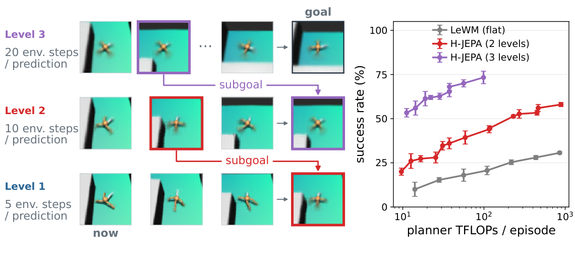
The widget shows what this buys in reach. Pick an environment and a depth and it draws, in environment steps, how far each level plans on the first call, using the horizons from the paper's planning table. A flat LeWM on AntMaze has to roll its single predictor 23 steps, 115 environment steps, and differentiate through all of it. A three-level model reaches 100 environment steps with five predictions at the top, and while the top is still planning, each level below rolls out only two steps.
- H-JEPA success
- 73.3%
- HWM success
- 38.7%
- flat LeWM
- 18.0%
- training clips vs LeWM
- 88%
Visual AntMaze: expert route between cells three apart, 82 steps on average, episode budget 350 steps. H is the configured horizon from the paper’s Table 7. On the first call the top active level plans its full H; every level below it plans two steps, just enough to reach the first subgoal it is handed. Later calls shrink the top horizon toward one, and an upper level whose horizon is one is skipped.
So the compute story is about depth of rollout. Gradients through two predictor steps are cheap and well-behaved; gradients through 23 autoregressive steps of a model that has compounding error are neither. The planner budget in the depth comparison is capped at 100 TFLOPs per episode for every model, which is what makes the comparison fair.
The result, and the two levers inside it
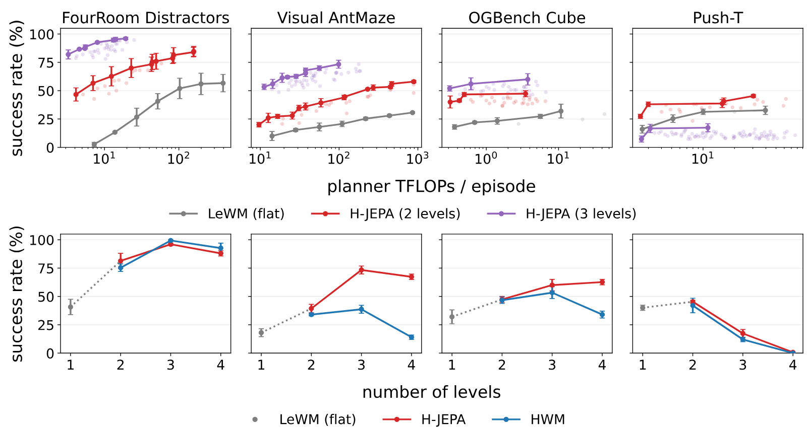
On FourRoom, AntMaze and Cube each added level up to three moves the Pareto front up and to the left: more success for less planner compute. On AntMaze, under the 100-TFLOP cap, flat LeWM solves 18.0% of the 50 tasks, two-level H-JEPA 39.3%, three-level 73.3%. Cube goes from 32.0% to 60.0% at three levels. FourRoom goes from 40.7% to 96.0%.
The comparison I care about is the blue line, because it answers "is this just HWM again?" HWM is the same group's earlier hierarchical planner: one latent space, several prediction horizons. The authors rebuild it inside this codebase as H-JEPA with identity encoders above level 1, so the two differ only in whether the upper levels get a representation of their own. On AntMaze the difference is large: three-level HWM reaches 38.7% against H-JEPA's 73.3%, and four-level HWM falls to 14.0%. On FourRoom it vanishes, and HWM is actually ahead at three levels, 99.3% against 96.0%. The checkpoints confirm this is a fair fight in size: the identity encoders save only 1 to 4 MB per AntMaze model (93.4 MB against 94.6 MB at two levels), because the predictors dominate.
So there are two things in a hierarchy, and Section 4.2 pulls them apart.
The first is the cost. The authors take each trained H-JEPA, throw away its upper planners, and plan flat with level 1 only, changing nothing except where the distance to the goal is measured: in level-1 space, or after pushing both the prediction and the goal up through the upper encoders. The rollout dynamics are identical. Only the ruler changes.
| AntMaze success (%) | 2 levels | 3 levels | 4 levels |
|---|---|---|---|
| Flat planning, native level-1 cost | 23.3 | 16.7 | 10.0 |
| Flat planning, best upper-level cost | 31.3 | 22.0 | 26.7 |
| Full hierarchical planner | 39.3 | 73.3 | 63.3 |
Measuring distance in a more abstract space helps a flat planner at every depth, and the best projected cost beats the separately trained LeWM's 18.0%. The cost maps show why. In level-1 space, the latent distance to a fixed point in the maze is nearly flat everywhere except right next to it, so a gradient planner has nothing to follow until it is already close. At levels 2 and 3 the distance rises smoothly along the corridors.
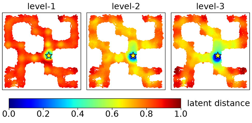
The second lever is time. A flat planner's cost to the final goal is a bad progress signal even along an expert trajectory: the paper measures its monotonicity, the negative Spearman correlation of cost with time, at 0.48 to 0.75 across the four simulated environments. The cost of tracking the next level-2 subgoal over a short segment scores 0.89 to 1.00 for H-JEPA. HWM gets nearly the same subgoal benefit, which is why it beats flat LeWM everywhere. The representation lever is what H-JEPA adds on top, and it only shows up where the frequency gap gave the upper levels something to throw away.
I like this section a lot. The cost-only ablation is the kind of experiment that tells a practitioner something usable today: if you already have a hierarchical encoder, you can get part of the gain with your existing flat planner by changing the ruler.
Where it does not help
The paper puts its failures in the main text, and they are instructive.
Push-T is the clearest. Two levels match or slightly beat LeWM, 45.3% against 40.0%. Three levels drop to 17.3% and four to 0.7%. The paper's explanation is data, and I think it is right. A training sample must fit inside one episode, and a four-level sample needs 25 level-1 frames, 121 environment steps. Push-T episodes average 125 steps, so a four-level model sees only 14% of the training clips LeWM sees per epoch, and three levels see 58%. HWM collapses the same way, which points at the data rather than the representation.
Cube is subtler. The full hierarchy helps there, 60.0% at three levels, but the cost-only ablation does not: the level-2 cost lowers the two-level model's flat success from 24.0% to 13.3%, and the level-3 and level-4 costs roughly halve success in the deeper models. With no frequency gap there is no useful abstraction to measure in, so whatever Cube gains comes from the subgoal lever alone. The authors say as much, and add that their results "do not establish that selective abstraction alone causes the gains in the other environments." A careful sentence, and I appreciated it.
Then the data-specialisation appendix, which deserves more attention than its position suggests. Trained end to end, both levels must see the same data. Trained stagewise, each level can have its own. On AntMaze, training level 1 on the noisy exploration data and level 2 on the goal-directed "stitch" data reaches 67% hierarchical success, while end to end on the union of both reaches 54%. The reverse pairing collapses to 2%. The low level wants coverage; the high level wants trajectories that go somewhere. End-to-end training cannot express that preference. The paper's headline recipe is end to end, but its own best AntMaze cell outside the main table came from not doing it.
DROID, and a collapse SIGReg cannot see
Every environment so far has a fixed camera and a fixed background. DROID does not: it is real teleoperated Franka video where the scene, lighting, camera calibration and objects change every episode. Train LeWM on it and planning fidelity is zero.
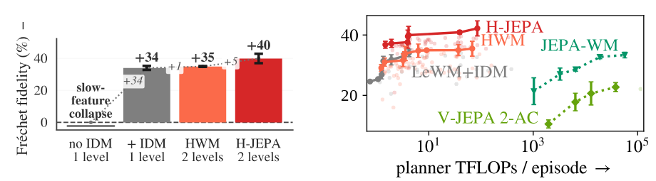
The appendix that explains this is the best writing in the paper. It names the failure slow-feature collapse: the encoder learns to encode only what is constant within an episode, the background, and ignores the moving arm. That solution has zero prediction loss, because the identity predictor is perfect when nothing changes, and here is the uncomfortable part: SIGReg cannot rule it out. Their Proposition 1 says it for any regulariser that only looks at the marginal distribution of single embeddings. If backgrounds vary continuously across episodes, you can map each background to a draw from exactly the target Gaussian. Every batch then looks perfectly isotropic, and the encoder still says nothing about the robot.
Recall the (T, B, D) grouping in the SIGReg code. Each test sees one timestep across many
sequences, and a collapsed encoder gives one distinct, Gaussian-looking embedding per sequence.
The "slow-feature collapse" button in the SIGReg widget above is exactly that case: the same
cloud as the healthy one, the same statistic, and nothing that moves when the robot moves. The
appendix measures where the variance actually goes in trained latents: 75% of it lies between
episodes on DROID against 28% on Cube.
They test two fixes. Putting time into the sample axis of the test adds a barrier, but a small one, and every run in their SIGReg sweep still collapses. A "time repulsion" term that rewards latents for changing keeps the predictor off the identity but never clears the zero-action floor. What works is an inverse-dynamics head that must regress the action from two consecutive latents. A collapsed encoder carries no information about the action, so the head's loss has a floor fixed by the data, 1 with normalised actions, which is 50 at the weight they use. The appendix calls it "the only barrier here," and notes the cost: it needs action labels. So the two-term recipe that works in simulation becomes, on real video, a three-term one: prediction, SIGReg, and action regression with weight 100 at level 1 and 50 at level 2.
With that term, the numbers are modest and honest. The paper's bars read +34 for flat LeWM plus inverse dynamics, +35 for HWM and +40 for H-JEPA, as medians over training and planner seeds. The README reports the same models as means: 33.57%, 35.65% and 38.42%. H-JEPA gets there at 10.1 planner TFLOPs per episode against 14.5 for the flat model.
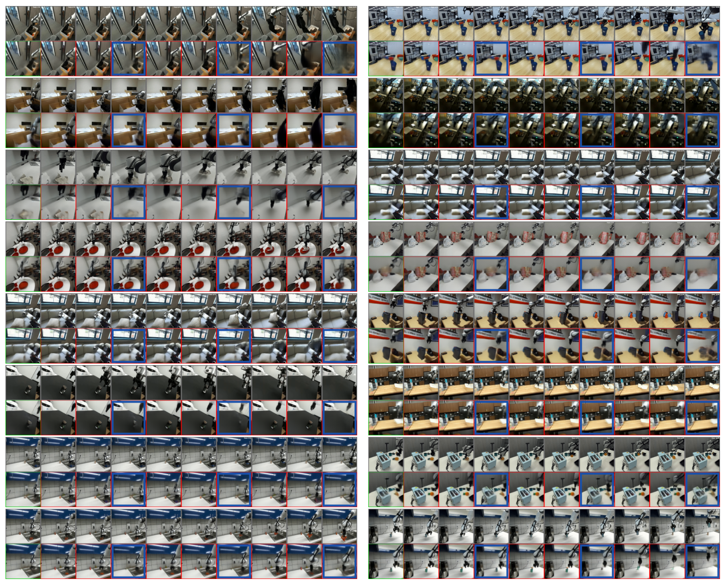
Two things limit how far I would take this. Fréchet fidelity is an offline metric: it compares the planned end-effector path with the logged expert path, with 0% meaning the arm does not move and 100% meaning it follows the expert. Nothing is executed on a robot. The paper calibrates the metric in simulation and concludes it is a necessary condition for success on Cube, not a predictor of it. Their conclusion states the open question plainly: "A next step is to test whether these gains translate to closed-loop control on a physical robot." And the evaluation is 16 hand-picked clips with good lighting and large objects. A careful protocol, and a small one.
Two replies worth reading
Two replies under the announcement point at work the article should mention. Daniel Korchinski linked his paper with Alessandro Favero and Matthieu Wyart, arXiv 2605.27734. It proves that on data from a probabilistic context-free grammar, latent prediction recovers a hidden tree with a sample count constant in its depth, where token-level learning needs exponentially many, and that data2vec already does this implicitly. Its abstract ends: "This suggests that explicit stacking such as H-JEPA is largely redundant." The theory is about static compositional data with no actions and no planning. H-JEPA's evidence agrees with it in one respect: on Push-T and Cube, where there is no separation of timescales, a separate representation per level adds little. Where the world has a slow part and a fast part, and a planner needs a ruler for the slow part, the explicit levels earned their keep. I do not think the two papers contradict each other; they disagree about which data matters.
The other reply links HDFlow, a hierarchical planner with a diffusion model proposing latent subgoals and a rectified-flow model filling in trajectories, and asks why this group never uses diffusion dynamics. Nobody had answered when I read the thread. My reading of the design is that a deterministic predictor is what makes gradient-through-the-rollout planning possible here; a stochastic generator would push you back toward sampling planners. I am inferring this; the authors have not said it.
What I would take from it
The idea that will last is the separation of the two levers. Measure distance where the dynamics are slow, plan in time where the horizon is long, and check which one your problem actually needs. The cost-projection experiment is cheap to run on any stack of encoders, and the frequency gap is a cheap thing to compute on a dataset before you build anything.
The part I would be careful with is "end to end" as a virtue. It works, it is stable, and SIGReg genuinely makes joint training of four latent spaces uneventful. But the paper's own appendix shows that training each level on its own data beat it on AntMaze, and that on real video the regulariser needs an action-supervised partner. The training is end to end; the safety net is not SIGReg alone.
And the real-robot claim should wait for a real robot. The simulation results are strong and well controlled. DROID is an offline proxy on 16 clips.
How I checked
I read the arXiv HTML of 2610.06805v1, including every appendix, and shallow-cloned
kevinghst/H-JEPA at commit 840e76b. Code quotes are from that commit with file and line. The
hierarchy, loss assembly, SIGReg quadrature, solver loop, macro-action clipping and per-level
configs were read from source; I did not run any of it. Checkpoint counts and sizes come from the
Hugging Face model API for jepa-world-models/h-jepa: 93 checkpoint files, 84 for simulation
and 9 for DROID, about 12.43 GB in all, matching the README's 9.7 GB and 2.7 GB. The SIGReg
widget is my own toy that reimplements the released formula on synthetic 2-D data; the depth
widget plots the paper's Table 7 horizons and the Figure 6 and Table 3 numbers.
A few things in the sources do not agree, none of them large. The four-level AntMaze hierarchical
result is 63.3% in the paper's Table 1 and 67.3% in Figure 6 and the README, so I quote the table
where I quote the table. The paper's DROID planning table lists 16 candidates at level 2, while
the released droid_l2.yaml and the README use 4. The DROID training corpus is 74,530 episodes
in the paper and 74,896 in the README's file list. ARCHITECTURE.md still describes a Push-T
example with stride 3 and 25 frames per step, which matches no released config. I could not check
any number that depends on running the planner, including all success rates and fidelities;
those are the authors'.