2026-09-26 · 23 min · quantization · mixture-of-experts · inference-optimization · offloading · llm · explainer
On 22 September Tim Dettmers announced a "runtime dynamic compression framework that achieves 1.5-2.0 bit compression at high quality", integrated into bitsandbytes2, "which starts as a private beta today". The paper is Runtime Dynamic Compression of Mixture of Experts: twelve pages, one author at Carnegie Mellon, set in the ICLR 2026 template while calling itself "the current version of this draft".
I read it end to end, digitized its result plots from the PDF's vector paths, and took apart the one piece of bitsandbytes2 anyone can download. The short version: this is not a new quantizer. It is an allocator and a runtime for mixture-of-experts (MoE) models. Offline, it picks a codec for every layer from a 13-rung ladder, and a fraction of that layer's experts to drop. At runtime it keeps changing which experts are resident. And "bits per weight" means resident bytes divided by all of the model's parameters. The experts that are not resident still exist, in CPU memory or on an NVMe disk, waiting to be swapped in.
What is decided offline, and what at runtime
"Runtime dynamic" is easy to over-read. Here is the split, from Sections 3 and 5:
| Decision | When | How |
|---|---|---|
| Codec per layer, 0.7 to 5 bits per weight | offline | iterative sensitivity probing and a Lagrangian allocator |
| Fraction of each layer's experts kept resident | offline | the same allocator, the same byte budget |
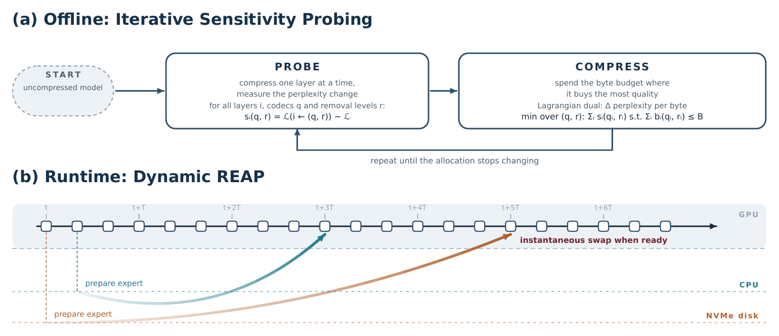
| Which experts are resident in each layer | runtime, every 256 tokens | dynamic REAP, up to four swaps per layer |
| Codec and count of resident experts | fixed | swaps keep "the expert count and codecs fixed" |
| Bit width per token or per request | never | — |
No per-token bit allocation, no codebook that changes at runtime. One byte budget is spent on two axes, how precisely each layer is stored and how many of its experts sit in fast memory, and only the membership of the second moves while the model runs.
Why static quantization runs out below 2 bits
Dynamic, or mixed-precision, quantization spends more bits on sensitive layers and fewer on the rest. Unsloth's dynamic GGUFs are the paper's reference point; I have audited one layer by layer for GLM-5.3-Flash. For dense models the paper calls this "largely solved": in its Figure 2, on a dense Qwen 3.8 27B, bnb2, QTIP, Unsloth and GSQ-RCO sit nearly on top of each other above 2.5 bits.
Below 2 bits, three things break.
Sensitivities stop adding up. An allocator needs a cost per layer, and the cheap way to get one is to compress one layer at a time on an untouched model. That works while compression is mild: "degradations remain additive under weak compression but become super-additive under strong compression". A layer that looks insensitive beside 16-bit neighbours can be the one that tips the model over once those neighbours are at 1.5 bits.
The ladder is too coarse. With codecs at 1, 2, 3, 4 and 5 bits, a layer whose sensitivity jumps between 1 and 2 bits has nowhere to sit. The paper blames this for QTIP's weaker showing: fractional QTIP codecs are possible, but encoding a matrix "can take days of GPU time".
Quantization alone does not reach the device. A 552B model at 2 bits is 138 GB of weights (my arithmetic). The paper's answer is a second axis, removing experts, without freezing the removal.
The codec: rotate, then look up a Gaussian codebook
bnb2 quantizes with HIGGS (Malinovskii et al.). A randomized Hadamard rotation spreads outliers across a block so the rotated weights look Gaussian, and a fixed codebook built for Gaussian vectors encodes them. It is the rotate-first idea behind TurboQuant, applied to weights with vector codes: a -dimensional group of weights becomes one -bit index, the rate is bits per weight, and fractional rates come for free. The paper's ladder:
The paper prints no kernel, but the bitsandbytes-kernels wheel on PyPI (more on it below) has a
quantize_vq_l2 that does exactly this:
# bitsandbytes/functional.py, bitsandbytes-kernels 0.50.0.dev0 (abridged)
W_blocks = W.reshape(N, n_rot, R)                    # R = 1024 by default
l2_norms = W_blocks.norm(dim=2).clamp_(min=1e-12)    # one scale per row per block
W_unit = W_blocks / l2_norms.unsqueeze(2)
W_rot = W_unit.reshape(N * n_rot, R).to(torch.bfloat16)
_apply_hadamard_vq(W_rot, R, signs=signs)             # sign flip, then Hadamard
W_rot = W_rot.float() * (R**0.5)                      # to unit-Gaussian scale
# ...
packed, _ = quantize_vq_bitplane(vq_flat, p=p, codebook=codebook, index_bits=index_bits)
l2_scales = l2_norms.to(torch.float16)
That makes the overhead easy to count. One fp16 norm per 1,024 weights is
bits per weight, and the codebook is shared rather than stored per layer. The wheel's own
allocator adds exactly that, scale_overhead = 16 / rot_blocksize, to every codec's rate. It
lists 22 weight codecs, vector length 2 to 16 and index 4 to 20 bits, at 16 distinct rates from 1
to 5 bits. There is no 0.7-bit rung, and the paper's ladder has 13 rungs while its Section 4 prices
"16 codecs"; the wheel looks like an earlier cut of the same system.
The rotation also makes allocation cheap. After it, a layer's quantization error is its weight variance times a constant of the codebook. The wheel ships those constants, measured on Gaussian data: 0.429 at 1 bit, 0.201 at 1.5, 0.094 at 2, 0.026 at 3 and 0.0068 at 4, within a factor of 1.5 to 1.7 of the Gaussian bound from 1 to 4 bits (my arithmetic). The paper fits its ladder with
and notes that is close to the 2 in the ideal Gaussian law . It is a fit, not a literal error: read as a normalized squared error, would be worse than rounding every weight to zero. What matters is the consequence. If distortion follows from the bit width alone, each layer only has to be probed at two codecs, and the rest interpolates.
Iterative sensitivity probing
Section 3.1 turns allocation into a loop. At iteration the model has a configuration that gives each layer a codec and an expert-removal fraction . A layer's sensitivity to a setting is measured on the whole model, every other layer left where it is:
is log-perplexity on a calibration set (RedPajama). With the bytes layer needs at a setting and the budget, the allocation is
A multiplier prices every byte in units of log-perplexity. For a fixed each layer chooses on its own,
and the dual search raises until the total fits. Settings are discrete, so the result "need not consume every available byte".
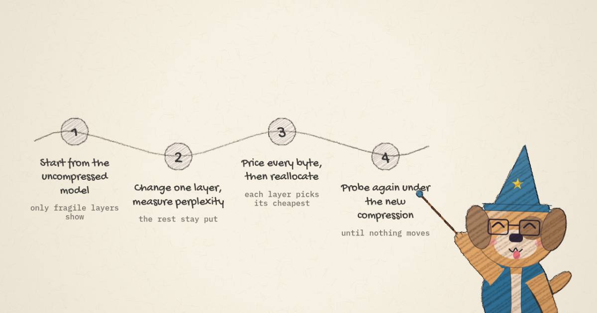
The chicken and egg is in . Sensitivities are only honest near the "edge of instability", where nothing has collapsed yet but any further compression would, and you only get there with a good allocation. ISP iterates its way there. Probe the uncompressed model, which only exposes the catastrophically fragile layers. Compress what looks safe. Re-probe under that compression, which exposes the next set. Stop when the allocation stops changing. The toy below runs that loop on the paper's ladder and distortion law, with twelve invented layers and an invented interaction between neighbours:
- uniform (1.25 everywhere)
- toy loss 6.981
- probe once (round 1)
- toy loss 7.629
- ISP, round 2
- toy loss 6.799
Re-probing under round 1's allocation moved 7 of 12 layers (solid bars). It evens out neighbours that were both pushed low, because now each probe sees them compressed together. The price of a bit, the multiplier λ, settled at 1.335 toy-loss units.
Illustrative: the layer amplitudes and the neighbour term are invented. The ladder, the distortion law and the probe-then-allocate loop are the paper's.
At a 1.25-bit budget the toy shows the failure plainly. Probing once on the uncompressed model gives a worse allocation than uniform 1.25 bits, toy loss 7.63 against 6.98, because it happily puts adjacent layers at 0.7 and 1 bit. The second round probes under that allocation, sees those neighbours compressed together, evens them out, and lands at 6.80. At 2.5 bits one round is enough: costs there are still additive.
Probing is the expensive part: ten codecs and ten removal levels are 100 evaluations per layer, which the paper says adds up to hundreds of GPU hours per ISP iteration. Two shortcuts from Section 4 cut that down. Only the extreme codecs are probed, 0.75 and 4.0 bits, and everything between is interpolated through . And the cost of removing a fraction of a layer's experts, , is modelled as a power law with one exponent for the whole network and one amplitude per layer:
It is fitted on three removal levels (none, 25% and 95%) and recovers the allocation with a Spearman correlation of about 0.9. That leaves 2 × 2 probes per layer plus one baseline, where 16 codecs and 20 removal levels would need 320: the "80x less computational cost" is 320 / 4. The runs use two ISP rounds; for GLM-5.3-Flash and DeepSeek-V4.1 the budget is annealed from 4.5 bits to 2.25, then 2.
The text is not fully consistent here: one description probes removal at 5% and 95%, the formal one at 25% and 95%, and the lowest probed codec is 0.75 bits on a ladder that starts at 0.7. It is the texture of a draft, not a change of method.
Dynamic REAP: the part that runs
REAP (Lasby et al.) prunes MoE experts in one shot. For expert in layer it averages the gate-weighted output norm over the calibration tokens that route to it,
keeps the best, and deletes the rest. Altar-1 is what that looks like shipped: GLM-5.3 with 168 of its 256 routed experts kept. Routing is confined to the resident set by masking the router logits before top- selection, for .
Dynamic REAP keeps the mask and changes its membership:
- The router computes logits for every expert anyway, so each expert's unmasked routing probability is tracked whether it is resident or not. Non-resident experts collect evidence without being run.
- Two exponential averages smooth it, with and half-lives of 100 and 1,000 tokens. The rank is their mean.
- Every 256 routed tokens, non-residents in descending rank are paired with residents in ascending rank. If at least four pairs have an incoming score more than 5% above the outgoing one, the first four are exchanged. Otherwise nothing moves, "to prevent thrashing". Swapped experts sit out until the next checkpoint.
- Incoming experts are prepared asynchronously from CPU memory or NVMe and swapped in at a decode-token boundary when ready, so no token waits for a transfer and the resident budget never grows.
The paper's evidence for the runtime half is a hit-rate grid on Qwen3.6-35B-A3B at 50% residency, 128 of 256 experts per layer. Calibrate the resident set on one domain, evaluate on another, and count the share of routing probability that lands on resident experts:
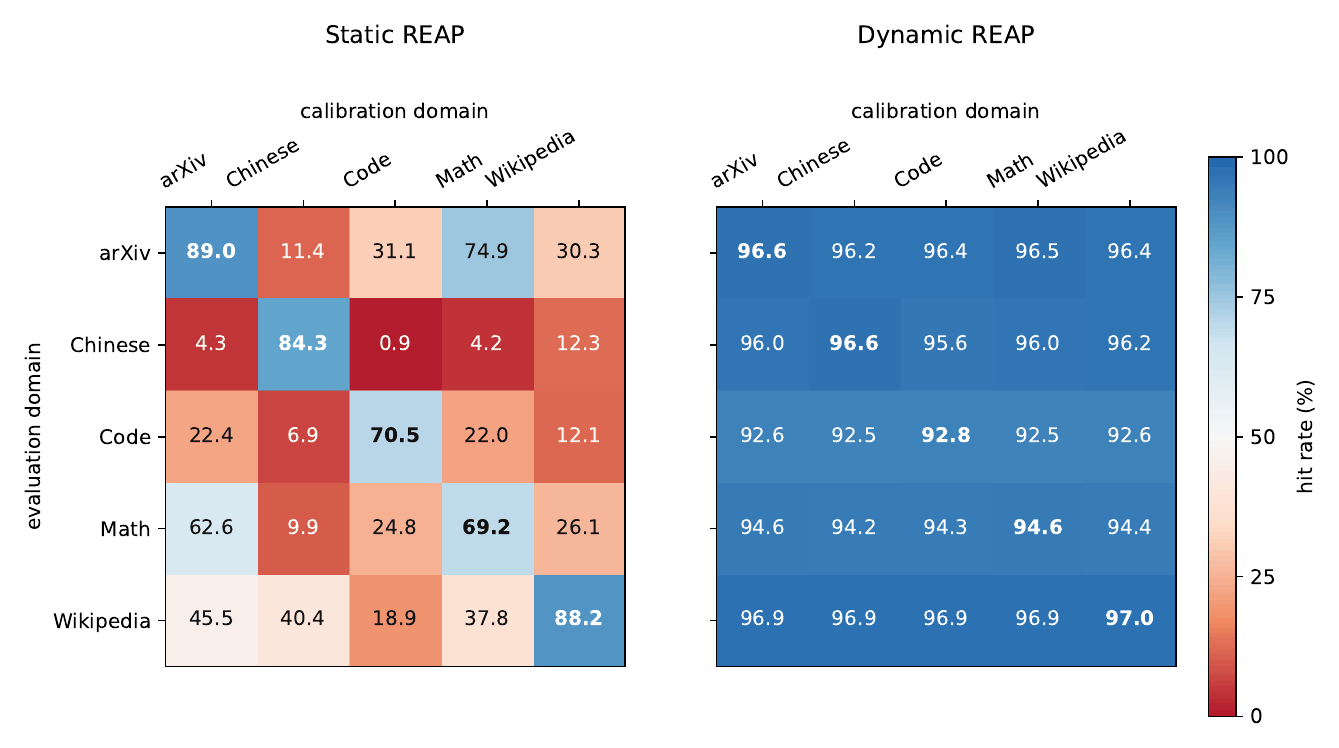
Static REAP is good on its own domain, 70.5% to 89.0% on the diagonal, and poor almost everywhere else: the Code-calibrated set catches 0.9% of the routing mass on Chinese text. Dynamic REAP holds 92.5% to 97.0% on all 25 pairs, and beats static REAP even where static was calibrated on the test domain. That last part is the interesting one. Routing drifts within a document, so the average routing over a dataset is a poor proxy even for that dataset.
Two limits. Hit rate is routing coverage, not quality; the paper reports no perplexity for static against dynamic REAP. And it reports no transfer volume or bandwidth for the swaps, which is the cost the design exists to hide. Four swaps per 256 tokens replace at most 3.1% of a 128-expert resident set per checkpoint; how many bytes that is depends on expert size, which the paper does not give.
The toy below implements the swap rule as written, on a synthetic 32-expert layer and a stream of four "domains":
| hit rate | A | B | C | D | all |
|---|---|---|---|---|---|
| static | 94.2% | 28.9% | 78.2% | 35.9% | 59.3% |
| dynamic | 94.2% | 80.7% | 85.9% | 86.8% | 86.9% |
The static set is right only on its own domain. The dynamic set starts from the same experts, and after each shift it climbs back in steps of four swaps per checkpoint, lagging by the time the running averages need to notice. More residency helps both; it helps static REAP only where its calibration domain overlaps the traffic.
Illustrative: synthetic routing, 32 experts, one layer. The swap rule is the paper's; the percentages are not.
With 16 of 32 experts resident and the static set calibrated on domain A, the toy's static hit rate falls from 94.2% on A to 28.9% on B. The dynamic set recovers to 80.7% on B and averages 86.9% against 59.3% for static, after only four swap events, because a few experts carry most of each domain's routing mass. The numbers are the toy's; the shape is the point.
The results, read off the vector plots
The paper reports results only as plots, so I digitized them: PyMuPDF returns each matplotlib marker as a filled path whose centre is the data point, and the gridlines calibrate the axes. The Unsloth footprints come back as 2.13, 2.32, 2.54, 2.95, 3.15 and 3.89 bits, a good sign the calibration is right.
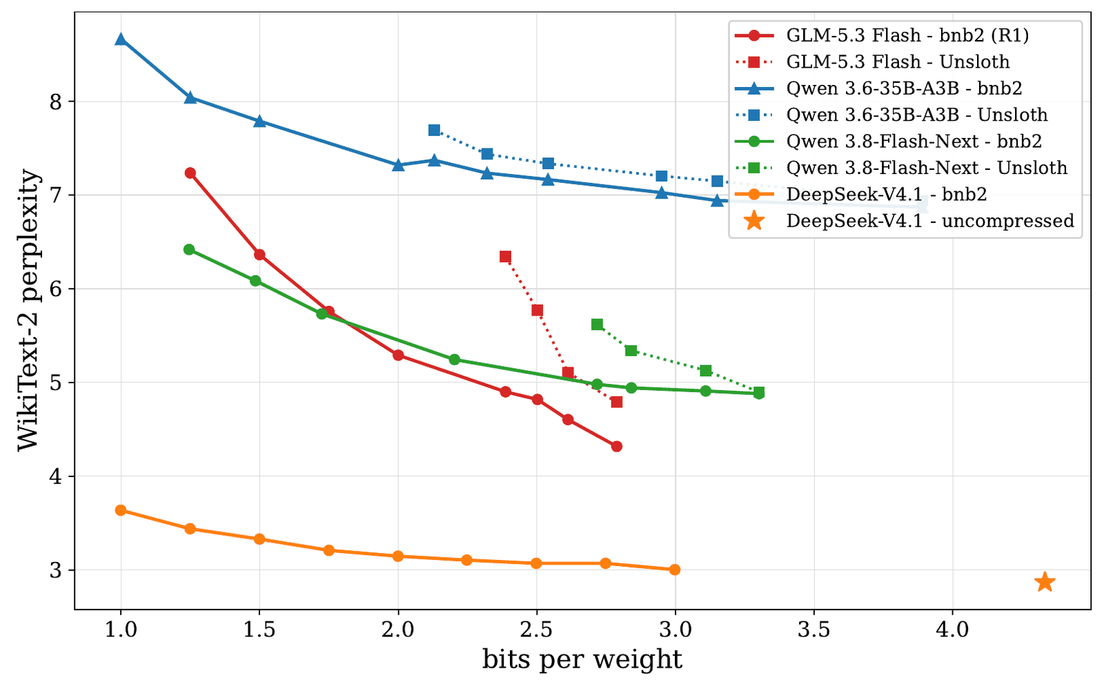
Evaluation is WikiText-2 perplexity through llama.cpp's standard tool, in 512-token chunks with the last 256 scored. bnb2 is allocated to each Unsloth checkpoint's footprint, then run with dynamic REAP swapping four experts per layer every 256 tokens. For each Unsloth point there are two readings: bnb2's perplexity at the same bits, and the bits bnb2 needs to match Unsloth's perplexity, which is my linear interpolation along the bnb2 curve.
Unsloth at 2.72 bits scores 5.62. At the same footprint bnb2 scores 4.98 (−11.4%). bnb2 reaches 5.62 at 1.84 bits: 0.88 bits fewer per weight.
Reported perplexities, digitized from the PDF's vector plot; the equal-quality crossing is my linear interpolation between plotted points. bnb2 bits count resident weights only.
| Model | Unsloth bits | Unsloth ppl | bnb2 ppl, same bits | bnb2 bits, same ppl | Gap |
|---|---|---|---|---|---|
| Qwen3.6-35B-A3B | 2.13 | 7.69 | 7.37 | 1.60 | 0.53 |
| Qwen3.6-35B-A3B | 2.32 | 7.44 | 7.23 | 1.88 | 0.45 |
| Qwen3.6-35B-A3B | 2.54 | 7.34 | 7.17 | 1.98 | 0.56 |
| Qwen3.6-35B-A3B | 2.95 | 7.20 | 7.03 | 2.42 | 0.53 |
| Qwen3.6-35B-A3B | 3.15 | 7.15 | 6.94 | 2.59 | 0.56 |
| Qwen3.6-35B-A3B | 3.89 | 6.94 | 6.87 | 3.20 | 0.69 |
| Qwen3.8-Flash-Next | 2.72 | 5.62 | 4.98 | 1.84 | 0.88 |
| Qwen3.8-Flash-Next | 2.84 | 5.34 | 4.94 | 2.11 | 0.73 |
| Qwen3.8-Flash-Next | 3.11 | 5.13 | 4.91 | 2.43 | 0.68 |
| Qwen3.8-Flash-Next | 3.30 | 4.90 | 4.88 | 3.19 | 0.11 |
| GLM-5.3-Flash | 2.39 | 6.34 | 4.90 | 1.51 | 0.88 |
| GLM-5.3-Flash | 2.50 | 5.77 | 4.82 | 1.75 | 0.76 |
| GLM-5.3-Flash | 2.61 | 5.11 | 4.60 | 2.18 | 0.43 |
| GLM-5.3-Flash | 2.79 | 4.79 | 4.32 | 2.52 | 0.27 |
Perplexities are the paper's, digitized; the last two columns are my interpolation.
The abstract says bnb2 lands "about 0.4 to 1 bit per weight below Unsloth". On the plotted points the gap is 0.11 to 0.88 bits: widest at the low end of each Unsloth ladder, narrowest where the curves converge. No point reaches a full bit. The paper's worked examples round in its favour: it pairs Unsloth's Qwen 3.8 Flash Next at 2.7 bits with bnb2 at 1.7, where I get 1.84, and Qwen 3.6 at 2.2 with 1.5, where I get 1.60. Its GLM example, 2.8 against 2.5, I reproduce at 2.52, and that is a 0.3-bit gap, under the abstract's own floor.
At matched footprints the picture is stronger. At 2.39 bits GLM-5.3-Flash scores 4.90 under bnb2 and 6.34 under Unsloth, 22.7% lower. GLM is also the paper's stated failure: its bnb2 curve climbs steeply below 2 bits, to 7.24 at 1.25, and the limitations section says dynamic compression of it "was not very successful". The paper also suggests that models with large "engram" tables, 51B parameters in Qwen 3.8 Flash Next (its N-gram embeddings) and 196B in DeepSeek-V4.1, degrade less when heavily quantized, in line with the precision scaling laws. The plot supports that less than the sentence does. From about 2 bits down to 1.25, DeepSeek-V4.1's perplexity rises 9%, level with the engram-free Qwen 3.6 at 10%, and Qwen 3.8 Flash Next rises 22%.
DeepSeek-V4.1 has no Unsloth curve, only its own uncompressed point at 4.33 bits per weight and perplexity 2.88. At 4.33 bits it is not a 16-bit reference; presumably it is the checkpoint as released, which is already low precision. Against it, bnb2 is +26.3% perplexity at 1 bit, +15.6% at 1.5, +9.3% at 2 and +4.3% at 3. Whether 9% more perplexity at 2 bits counts as "high quality" depends on the workload, and WikiText-2 cannot say.
Figure 1 plots the same points against gigabytes, with device lines. Dividing each point's size by its bits per weight gives one constant per model, 34.7B, 128.8B, 312B and 566B weights' worth, close to the 35B, 125B, 320B and 552B the text names. So the size axis is weights and nothing else.
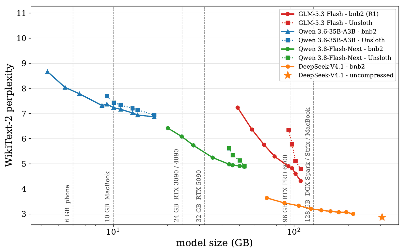
Read that way, the headline pairings are:
- Qwen3.8-Flash-Next in 24 GB. The 1.49-bit point is 23.91 GB at perplexity 6.09. On a 24 GB card that leaves under 0.1 GB for KV cache, activations and the runtime. The 1.25-bit point, 20.05 GB at 6.42, leaves about 4 GB.
- DeepSeek-V4.1 in 96 GB. The 1.25-bit point is 88.41 GB at 3.44. The 1.5-bit point, 106.12 GB, does not fit. Under the 128 GB line, the 1.75-bit point is 123.84 GB at 3.21.
What the paper does not measure
- Anything but perplexity. WikiText-2, one tool, no downstream tasks. KL divergence was skipped because the logits would take 130 GB of disk per model; the stated correlation between KLD and perplexity is r = 0.992 in Section 5 and r = 0.98 in Section 8. The limitations section concedes that the community finds "KLD and perplexity evaluations are not enough", and that out-of-distribution behaviour is what usually breaks.
- Most baselines. For the MoEs the only comparison is Unsloth. QTIP and GSQ-RCO appear only on the dense 27B; RCO's MoE checkpoint was uploaded "3 days ago" and is not compared. GPTQ, AWQ, QuIP#, AQLM and SpQR are related work only, and HQQ and BitNet-style ternary models do not appear. Ternary weights trained for the purpose are a different bet: see Bonsai 2 27B and Ternary15M.
- Speed. No throughput, latency or transfer-bandwidth number appears anywhere in the paper. Figure 3's caption says dynamic REAP incurs "practically no runtime speed overhead", unmeasured. The one speed figure is in the launch post: Qwen 3.6 35B-A3B "at 450 tokens per second" at 1.5 bits on the Mac and Metal build, with no machine, batch size or context length.
- The reservoir. Bits per weight count resident weights. Non-resident experts must live where a swap can reach them, and the paper never says how large that copy is or at what precision. Since swaps keep codecs fixed, the natural reading is every expert at its layer's codec, which makes the full model larger than the headline number. On unified-memory machines, the 128 GB DGX Spark, Strix and MacBook line, CPU and GPU memory are one pool, so the reservoir has to be the disk. It is the point I made about WanGP: a small resident number is a residency policy.
- Embeddings and KV cache. Related work faults other allocators because "none prices the embedding or LM head, none covers the KV cache". The method section does not describe how bnb2 does either.
What you can run today
The announcement is explicit that bnb2 is a private beta with limited places. Here is what is public:
- PyPI.
pip install bitsandbytes2resolves to0.50.0.dev0, uploaded 17 August 2026: a 1,221-byte metapackage that pins three others.bitsandbytes-kernelsis real: a 15.6 MB wheel for CPython 3.11 on x86-64 Linux only, with CUDA 12.1, 12.4 and 12.8 libraries and a CPU build. It holds the VQ-L2 quantizer above,fused_vq_l2_matmul_small_m, NVFP4 kernels anddynamic_bitalloc.py. Its README says Metal sources exist without a release library, and "AMD is later".bitsandbytes-cppcalls itself a "Python stub; native llama-server not in this TestPyPI wheel". The wrapper ships, with flags such as--expert-routing-profile,--expert-sensitivityand--expert-cold-nvmethat fit dynamic REAP, but thellama-serverbinary it launches does not, and neither does its model catalogue.bitsandbytes-code, the coding agent, is a stub that prints its version.
- The wheel's allocator is not ISP.
dynamic_bitalloc.pyis "data-free": a ridge regression over weight statistics, trained on Llama-2-7B, Llama-3.1-8B and Qwen3-8B, predicts each layer's sensitivity, and a greedy knapsack assigns codecs: "No calibration data or forward passes required". ISP is built on forward passes. - Models and source. I found no bnb2 checkpoints on Hugging Face. The GitHub repository named
in the PyPI metadata,
TimDettmers/bitsandbytes2, was not reachable from my session, which fits a private repository.
So today you can install kernels on Python 3.11 and quantize a matrix with VQ-L2. You cannot run the paper's system: no ISP, no dynamic REAP runtime, no compressed models. I read the wheel's source and did not run it; it is a dev build a month older than the paper, and the beta may differ.
Where it sits
Offloaders such as FreeToken, which the paper cites, keep every expert and fetch the missing ones per token; Edge0 predicts them a token early to hide the read. REAP pays once, in quality, and never fetches. Dynamic REAP sits between: approximate, but fetching on a 256-token clock that keeps transfers off the critical path. And where scalar formats like NVFP4 win on hardware support, vector codes win on rate granularity, which is what a sub-2-bit allocator needs.
The takeaway
The contribution is not a better way to write a weight in 1.5 bits. It is two ideas about where the bytes go. Measure each layer's cost under the compression you actually plan to ship, because below 2 bits costs stop adding up. And stop treating expert removal as a decision made once from a calibration set: the router already scores every expert on every token, so keep the ones the current text wants resident and fetch the rest in the background. The evidence for both is thinner than the headline, one metric and one baseline, but the second idea has a clean receipt in Figure 5, and neither one depends on the codec.