2026-10-06 · 19 min · diffusion · multimodal · image-generation · video-generation · representation-learning · flow-matching
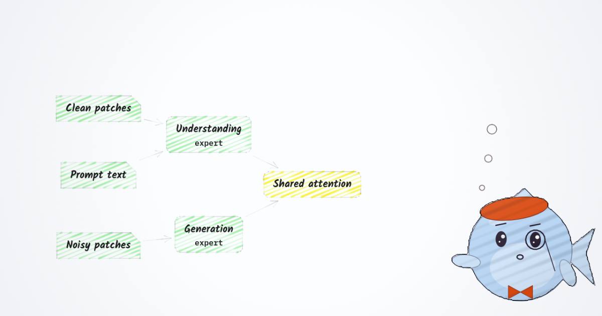
Two papers landed on arXiv within a day of each other, and both start from the same decision: no VAE. The diffusion model works on raw RGB patches.
- PixelUMM (NVIDIA and Waterloo) is a unified model. One decoder-only Transformer, initialised from Qwen3-8B, reads images and video, answers questions about them, and generates both. It has no vision encoder and no VAE. Pixels enter and leave through one linear layer each.
- PixelDense (Virginia, Michigan State, Adobe, Arcade AI) is a training recipe for pixel-space text-to-image denoisers. It adds four frozen perception models as alignment teachers during training, and drops them all at inference.
PixelUMM asks whether raw pixels can be a model's only visual interface. PixelDense asks what extra training signal a pixel denoiser needs. Both start from what the VAE was doing.
| PixelUMM | PixelDense | |
|---|---|---|
| What it is | unified understanding + generation, image and video | a training loss for pixel diffusion Transformers |
| Backbone | Qwen3-8B, every block split into two experts | PixelGen-XXL (1.1B) and DeCo (1.1B) |
| Visual interface | 16x16 patches, 4x16x16 tubes, one linear layer each way | 32x32 patches, 256 tokens at 512x512 |
| Headline (reported) | GenEval 0.77, or 0.83 with prompt rewriting; VBench total 83.24 | GenEval 0.7927 to 0.8093 on PixelGen-XXL |
| Release | code (Apache 2.0) and checkpoints, NVIDIA non-commercial licence | paper only, as of today |
Why latent diffusion used a VAE
A 512x512 RGB image is 786,432 numbers. Diffusion trains a network to denoise every one of them, at every noise level. Most of those numbers carry detail the eye barely notices: sensor grain, exact texture phase, the precise high-frequency content of a patch of grass.
Latent diffusion split the job in two. An autoencoder learns to compress the image 8 times per side and to decode it back. Diffusion then runs only in that compressed space, and the decoder restores the fine detail once at the end. The architecture doc on the Diffusion Transformer has the numbers: DiT-XL/2 in latent space used 118.6 Gflops against 1,120 for the pixel-space U-Net ADM, and won (reported there).
The VAE makes the problem cheaper and hands perceptually minor detail to a specialised decoder. It also costs three things:
- A reconstruction ceiling. The generator can never be sharper than the decoder. SenseNova-U1.5 measured how close a no-VAE model gets on COCO: 31.56 dB against Flux VAE's 32.65.
- A second training run that the generator has no say in.
- For unified models, a second visual stream. BAGEL, the reference unified model, feeds a ViT for understanding and a VAE for generation. PixelUMM's introduction says representing each conditioning image both ways "approximately doubles the visual context" (reported).
What pixel space has to solve
Drop the VAE and the first worry is sequence length. It turns out to be a non-issue. The real problem is token width.
A DiT on an 8x VAE with 2x2 patches makes one token per 16x16 pixels. A pixel model with 16x16 patches also makes one token per 16x16 pixels. At 512x512 both produce 1,024 tokens (reasoned). The difference is what each token holds: the latent token is 2 x 2 x 16 = 64 numbers, the pixel token is 16 x 16 x 3 = 768, twelve times more (reasoned).
The calculator above lays out the interfaces both papers use. Three rows matter:
- PixelUMM images: 16x16 patches, 768 values per token, fed into Qwen3-8B's 4,096-wide hidden state. The token fits comfortably.
- PixelUMM video: 4x16x16 tubes, 3,072 values per token, into the same 4,096 width. A 4-second, 24 fps, 512x512 clip is 96 frames and 24 x 32 x 32 = 24,576 tokens (reasoned), well under the 80K sequence length of the final training stage.
- PixelDense's backbone, PixelGen-XXL: 32x32 patches, 3,072 values per token, into a hidden width of 1,536 (reported, paper appendix A.1). Each token has twice as many numbers as the network that reads it.
That last row is only possible because of how these models choose their prediction target.
Predict the clean image, not the noise
Write the flow-matching corruption the way PixelUMM does, with clean and pure noise:
The network can be asked for three different things. -prediction outputs the noise. -prediction outputs the velocity . -prediction outputs the clean patch . They are algebraically interchangeable given and , so for years the choice looked like a matter of loss weighting.
JiT (Li and He) argued they are not interchangeable in practice. Natural images sit on a low-dimensional manifold inside the 768-dimensional patch space. Noise does not. To output or , the network has to reproduce every one of the 768 independent noise values, which a 768-to-hidden-to-768 Transformer with a bottleneck cannot carry. To output , it only has to name a point on the manifold. JiT's abstract says that at large patch sizes "predicting high-dimensional noised quantities can fail catastrophically" (reported).
PixelUMM follows JiT exactly. The head predicts , and the loss is computed in velocity space:
The clamp at 0.05 keeps the division from blowing up near clean data. I read the release code to check it is what ships: modeling/pixelumm/pixelumm.py sets x_pred_t_min=0.05 and refuses to build with a timestep embedding (measured, from the code). PixelUMM has no timestep input at all. The network infers how noisy a token is from the token, as MiniT2I does.
Patch size is the knob
Bigger patches mean fewer tokens and wider ones. PixelUMM ran this directly. With the same sequence-length budget, 32x32 patches fit four times as many images per step, yet the 16x16 run kept lower generation loss through training (reported, Takeaway 1). For video, of four tube shapes, the least compressed one, 32x32x1, reached the lowest loss. They shipped 16x16x4 anyway, to match the 4x temporal, 16x spatial convention of video VAEs like Wan2.2 (reported, Takeaway 2). Both shapes compress 1,024 pixels into one token.
PixelUMM: one backbone, two experts
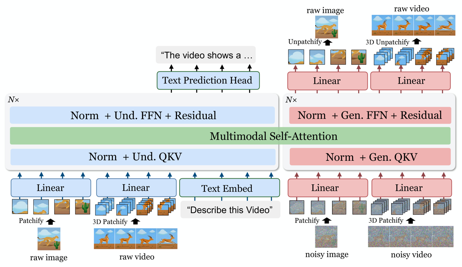
A Mixture-of-Transformers is not a mixture of experts in the routing sense. There is no learned router and no top-k. Each token's route is fixed by what it is: text and clean visual tokens take the understanding route, noisy visual tokens take the generation route. Each block holds two copies of the normalisation layers, the QKV and output projections and the FFN, one per route. All tokens still meet in one self-attention, so a noisy target patch can attend to the prompt and to clean reference images.
The code matches the figure: qwen3_navit.py defines a q_proj_moe_gen, k_proj_moe_gen, v_proj_moe_gen, o_proj_moe_gen, mlp_moe_gen and two *_layernorm_moe_gen next to every original Qwen3 layer (measured, from the code). That makes the parameter count predictable. Qwen3-8B is 8.19B parameters by its config. Duplicating all 36 decoder layers adds 6.95B, and the four pixel projections and two output heads add 47M. The total comes to 15.18B (reasoned). The model card lists 15,199,672,064, within 0.1% (reported). The released checkpoint is 30.39 GB of PyTorch distributed shards, two bytes per parameter, so bf16 (measured, from the Hugging Face file listing).
"8B" names what any one token passes through. The weights you download are almost twice that.
Three more details matter:
- The attention mask is block-causal. Text is causal. An image is one bidirectional island. Sparse video frames are ordered islands, so a later frame sees earlier ones but not the reverse. A noisy generation target sees the whole prompt and all of itself, and nothing before it can see into it.
- Video understanding has two modes.
dense_modesamples at 4 fps and uses tubes.sparse_modesamples at 1 fps and patches each frame like an image. At the same checkpoint the two were within 0.7 points of each other on every video benchmark (reported, Table 4), so the benchmarks use sparse mode.
Training runs in six stages over about 505K steps, starting at 256x256 and ending with a 20K-step joint stage at 512x512 for generation. The joint stage weights cross-entropy, image MSE and video MSE as 1:10:30 (reported, Table 1).
The findings worth keeping
The paper is candid about what went wrong. Two results stand out.
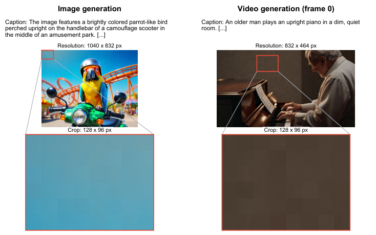
Patch artifacts. One linear layer back to pixels means every patch is decoded on its own, and nothing smooths the seams. At a classifier-free guidance of about 6, the grid shows. On a boundary probe over 72 prompts, the linear head's edges were 1.078x stronger at spatial patch boundaries and 1.160x at tube boundaries (reported). Convolutional PixelShuffle heads mostly fix it, at 5.6 to 9.6 times the head's FLOPs. The released model, the benchmarks and the demos all use the linear head, because switching needs more training. The paper says so plainly.
The pixel versus VAE comparison does not show what it seems to. At 10K steps the VAE-space loss was about 4.3x the pixel loss, and the authors note at once that losses in different spaces say nothing about which learns faster (reported, Takeaway 4). The targets differ too: -prediction against -prediction.
Checking "comparable"
The post that brought this to me said the model is comparable to open baselines. The paper says the same and adds that with different training data, the tables "cannot establish which architecture is superior". Here are the rows I would look at, all from the paper's own tables (reported):
| Benchmark | PixelUMM 8B | BAGEL 7B | Best other in table |
|---|---|---|---|
| GenEval, original prompts | 0.77 | ||
| GenEval, rewritten prompts | 0.83 | 0.88 | 0.90 (Lance, TUNA) |
| DPG-Bench | 85.74 | 85.07 | 88.32 (Qwen-Image) |
| VBench total | 83.24 | 85.11 (Lance) | |
| MMMU | 41.67 | 55.30 | 69.60 (Qwen3-VL) |
| MMStar | 53.99 | 70.90 (Qwen3-VL) | |
| CountBench | 94.30 | 82.50 | 89.80 (Qwen3-VL) |
| MVBench | 70.53 | 77.10 (PLM) | |
| Video-MME, no subtitles | 57.33 | 73.00 (Keye-VL-1.5) |
"Comparable" holds for generation. GenEval with rewriting is 0.05 behind BAGEL, DPG-Bench is ahead of it, and the VBench total of 83.24 sits just under HunyuanVideo (83.43) and Wan2.1 (83.69), two dedicated video generators. It holds for counting, where PixelUMM leads every model in the table, and roughly for MVBench, where it is mid-table. It does not hold for knowledge-heavy understanding: MMMU is 13.63 points below BAGEL and 27.93 below Qwen3-VL-8B (reasoned). No vision encoder means no inherited CLIP-style pretraining, and that is where it shows. Neither paper reports FID for text-to-image.

REPA, from first principles
Now PixelDense. To follow it, you need REPA (Yu et al., ICLR 2025).
A diffusion Transformer learns two things at once: what images contain, and how to remove noise from them. The first is slow to learn. Self-supervised encoders like DINOv2 already know it. REPA's move is to make an intermediate layer of the denoiser agree with such an encoder while it trains.
Take the denoiser's hidden state at block , one vector per patch token . Run the clean image through a frozen encoder to get one feature per patch at the same grid position. Push the denoiser's feature through a small projector , and pull it toward the teacher with a cosine loss:
The denoiser only ever sees the noisy image, so it has to learn to recover clean-image features from noise. The teacher and projector are thrown away after training, so sampling cost does not change. The REPA abstract reports SiT training sped up "by over 17.5×" (reported).
Two later results set up PixelDense. iREPA (Singh et al.) found that what transfers is the teacher's spatial structure, not its global semantics. And in pixel space, alignment is unusually direct: each denoiser token is a patch of the same RGB grid the teacher sees, so the alignment target is just the teacher feature at that location. If spatial structure is what helps, models trained to output spatial structure should be better teachers. Those are segmentation, depth and surface normal models.
PixelDense: two streams and an orthogonality penalty
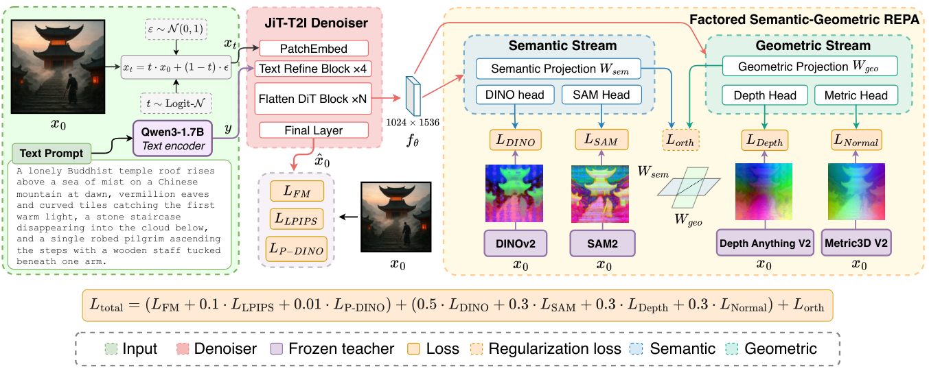
The paper's first finding is the motivation. On a PixelGen-XXL backbone that already aligns to DINOv2, adding any one dense teacher raises GenEval Overall from 0.7927. Depth Anything v2 helps most at 0.8069, then Metric3D v2 at 0.8060, then SAM2 at 0.8020 (reported, Table 3). The second finding is the problem: a flat sum of four teachers lands below the best single teacher, at 0.8036 GenEval Overall with equal weights, and lower under the two other weightings tried.
The paper's explanation is gradient interference. Semantic teachers reward invariance: the same object should look the same from any angle. Geometric teachers reward the opposite: where the surface is, which way it faces. Even with a separate projector per teacher, all four losses pull on the same denoiser feature , and those pulls can cancel.
PixelDense's fix has two parts.
Two streams. The token at block 8 (of 16) feeds a semantic stream and a geometric stream, each a two-layer MLP: . The semantic stream is 768 wide and feeds the DINOv2 and SAM2 heads. The geometric stream is 1,024 wide and feeds Depth Anything v2 and Metric3D v2. Teachers that agree share a bottleneck; teachers that disagree do not.
Orthogonality. Two streams alone do not guarantee separation, since both read the same . So the first-layer weights are pushed apart:
where has each row normalised to unit length. That is the mean absolute cosine between every semantic row and every geometric row. When it is zero, the two streams read orthogonal directions of , so their gradients enter the denoiser through separate subspaces. The penalty only touches weights, so it needs no data and costs nothing at inference. Its weight is ; the alignment losses are weighted 0.5 for DINOv2 and 0.3 for each of the others.
The penalty only constrains the first linear map, not the full nonlinear streams. The paper says so. It is a nudge toward separation, not a proof of it.
What the numbers show
The headline: GenEval Overall goes from 0.7927 to 0.8093 on PixelGen-XXL, a 2.09% relative gain, which I confirmed from the two numbers (reasoned). DPG-Bench moves from 78.7 to 78.9 and HPS v2.1 from 0.280 to 0.282 (reported, Table 1). On DeCo, with the recipe unchanged, GenEval goes from 0.8620 to 0.8690 (reported, Table 5).
The widget lays out the whole composition table. Two things stand out to me.
DINOv2 is still the anchor. Removing it costs the most of any teacher, down to 0.7940. The geometric stream alone, without DINOv2, scores 0.7960, below either geometric teacher paired with DINOv2. Dense teachers add to semantic alignment. They do not replace it.
The spread is small next to one run's noise. The table's rows span 0.7940 to 0.8093, 0.0153 wide. GenEval has 553 prompts. At four images per prompt, GenEval's usual setting, a binomial standard error at a score near 0.8 is about 0.0085 (reasoned; the paper does not say how many images it drew). Seed-matched sampling helps, since every row sees the same prompts and noise, but each row is still one fine-tune. The headline gap of 0.0166 is about two standard errors. The ordering of the middle rows, 0.8020 against 0.8027 against 0.8036, is not established by these runs.
The stronger evidence is elsewhere: the reconstruction probes.
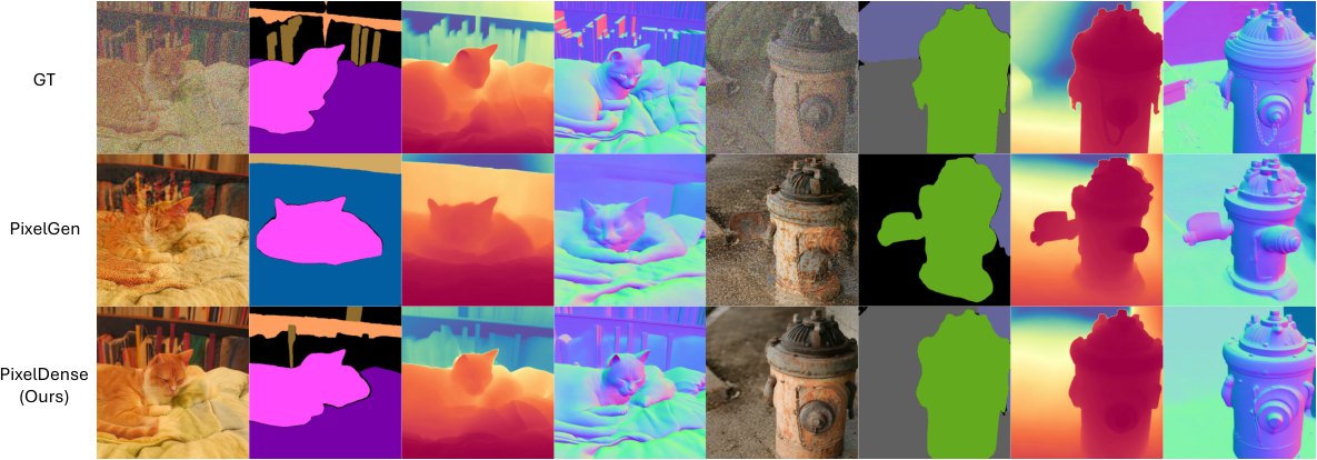
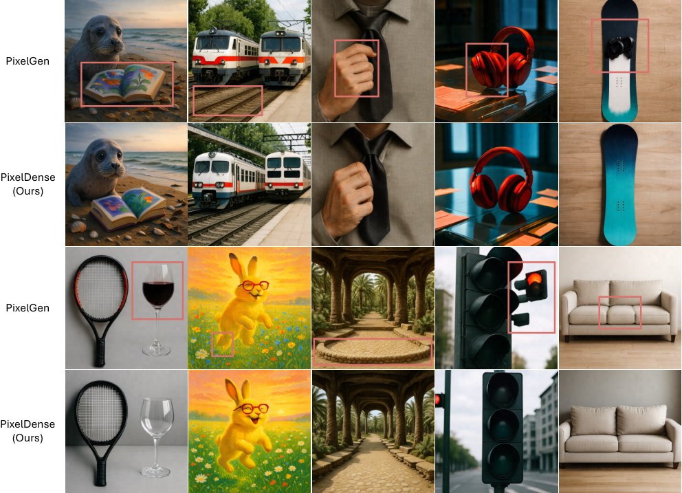
Noise a real COCO or Flickr30K image halfway, let the model denoise it with its caption, and score the result with OneFormer and Marigold, which are not among the training teachers. At , panoptic quality rises from 23.23 to 31.43 on COCO with real labels, and from 19.66 to 30.09 on Flickr30K. Those are the abstract's 35.3% and 53.1%; I recomputed both from Table 2 (reasoned). Depth error falls 36.0% on Flickr30K and 32.9% on COCO (reasoned, from the table). PixelDense wins every cell. In SDEdit editing on PIE-Bench, background PSNR is higher at every noise level, by 1.53 to 2.16 dB (reasoned, from Table 6), matching the abstract's "up to 2.2 dB".
That is what geometric teachers should buy: a model that keeps where things are. Small composition gains on GenEval are a side effect.
Two things in the paper that do not line up
- Token count. Figure 2 labels the denoiser feature 1024 x 1536. Appendix A.1 says 512x512 inputs, 32x32 patches, 256 tokens of width 1,536. 512/32 = 16 and 16 x 16 = 256 (reasoned), so the appendix is right and the figure's 1024 is the 16x16-patch count.
- Depth error units. Table 2's depth cells read 1.58, 1.06 and so on, called "AbsRel after per-image affine fitting". AbsRel is a fraction; a value above 1 means the error exceeds the depth. These are probably scaled, perhaps by 10, but the paper does not say. The relative improvements do not depend on the unit.
The 1.23x faster from-scratch convergence is read off a plot (Figure 4), at 128x128 resolution. I could not check it.
How the two papers fit together
They solve different halves of the same move. PixelUMM shows that a unified model can drop both visual encoders and still generate competitive images and video, provided it predicts clean pixels. Its weak spot is understanding that depends on visual pretraining. PixelDense shows that a pixel denoiser can be given that pretraining back at training time, through alignment, without carrying any of it into inference.
PixelUMM does not use REPA. Its generation expert learns pixels from the flow loss alone. The obvious question is whether PixelDense's teachers, aligned at the generation expert's middle layers, would close some of PixelUMM's gap. Neither paper tests it, so that is a question, not a claim.
Related reading on this site: CSFM on what the flow-matching source distribution could be, GAE for geometry generated alongside RGB rather than distilled into it, Marigold V2 for another alignment loss aimed at a perception target, and Inkling for encoder-free inputs in a much larger model.
What I would want next
- PixelUMM with a convolutional head. The released model knowingly ships the grid artifacts. A PixelShuffle head was the paper's own best trade-off.
- Seeds for PixelDense. Three fine-tunes per row of the composition table would show which differences are real. The probes are convincing; the GenEval ordering is not yet.
- A matched pixel versus VAE comparison in image quality, not loss. PixelUMM measured the loss gap and correctly declined to interpret it. The quality comparison is the one that would settle the question.
Sources
- PixelUMM paper: arXiv 2609.38597 · project page · model card (base model
Qwen/Qwen3-8B) · codenv-tlabs/PixelUMM, read at commite19e91a - PixelDense paper: arXiv 2610.00483
- REPA: arXiv 2410.06940 · JiT: arXiv 2511.13720 · iREPA: arXiv 2512.10794
- Qwen3-8B config: huggingface.co/Qwen/Qwen3-8B (hidden size 4,096, 36 layers)
- Wan2.2 VAE config: Wan-AI/Wan2.2-TI2V-5B-Diffusers (48 latent channels, 16x spatial, 4x temporal)