2026-09-22 · 27 min · 3d · point-cloud · diffusion · world-models · depth-estimation · open-weights · explainer
The usual way to get 3D out of a video generator is to generate the video and then run a reconstructor on it. Frames out of the diffusion model, VGGT or Pi3 or DA3 over the frames, point cloud out the other end. It works, and it is derivative by construction: the geometry can only ever be as good as a reconstructor's reading of a synthetic image, and every artefact the generator invents becomes a surface the reconstructor dutifully places in space.
GAE, from ARC Lab at Tencent and HKUST, makes a different bet. It generates in a latent that a geometry foundation model can already read, and pulls both appearance and 3D out of the same generated state. The project page puts it as a choice about where generation happens: put geometry inside the generated latent rather than around an appearance-only one as an external constraint, so that "every generated latent decodes into appearance and 3D — without reconstructing geometry as an afterthought." The showcase point clouds, they say, are native: decoded from the latent, not reconstructed from the generated RGB.
That is the whole article, because it is a checkable claim about a graph. If the geometry decoder reads only the same latent the RGB decoder reads, and never the decoded RGB, the architecture supports it. If the point cloud is assembled from pixels somewhere downstream, it does not. I read the forward path in the released code; below is which.
The claim is a graph question
Three files answer it.
The public API is a thin wrapper, and its two decode methods have the whole argument in their signatures:
# gae/pipeline.py — both take z, neither takes the other's output
def decode_rgb(self, z, num_views=None):
    rgb = self.codec.decode_rgb(z, num_views=num_views)
    return self._denormalize_rgb(rgb)

def decode_geometry(self, z, height, width, backbone_norm=None):
    decoder = getattr(self.backbone, "rae_cl_decoder", None)   # frozen DA3 DPT head
    recon = self.codec.decode(z)
    feats = self.codec.denormalize_and_split(recon)
    dpt_in = _format_recon_for_dpt(feats, backbone_norm, z.shape[0])
    return decoder(dpt_in, height, width, patch_start_idx=0)
One level down, in the codec itself, the two readouts share a decoder trunk and then fork:
# src/stage1/gae_codec.py
def decode(self, z):                       # → the four DA3 levels, for the DPT head
    seq, h, w = self._decode_trunk(z)
    c = seq.shape[-1]
    return self.dec_conv(seq.permute(0, 2, 1).reshape(-1, c, h, w))

def decode_rgb(self, z, num_views=None):   # → pixels
    seq, h, w = self._decode_trunk(z)
    return self.rgb_head(seq, h, w, num_views=num_views)
Shared trunk, two heads, and no argument passing between them. That matches the paper's Equation 7, which writes the two readouts as siblings of one state rather than a chain.
The third file is where a point cloud is actually built, and it is the one that would give the game away if the claim were marketing. In the evaluation and demo path, every point's coordinates come out of the decoded ray and the decoded depth, in one line:
# scripts/eval/eval_generation.py — _recover_view_pointclouds()
ray_np = _ray_to_numpy(ray)               # (V, H, W, 6): [direction | camera centre]
d_hw   = depth_tensor.float()...          # (V, H, W)   : decoded metric depth
points = ray_np[..., 3:] + d_hw[..., None] * ray_np[..., :3]
...
cols = (rgb_hwc[::stride, ::stride][valid] * 255.0).clip(0, 255).astype(np.uint8)
Origin plus depth times direction. The RGB tensor appears four lines later,
resized to the ray grid, and is used for exactly one thing: cols, the colour
written into each point. Delete the RGB head entirely and the point cloud's
geometry is unchanged — you get a grey cloud in the same places. The comment
above that function is explicit that this is a deliberate choice: recover_poses
is still run on the decoded ray to keep DA3's official camera convention, but
coordinates are built from the ray's own origin and direction rather than
back-projected through recovered intrinsics, because mixing the two gauges makes
the clouds drift.
z and nothing else. The point cloud is built from the DPT head's own ray and depth output; RGB enters only as the colour written into each point.So: the geometry decoder is independent of the RGB decode path. The information flows latent to geometry and latent to appearance, never appearance to geometry. The paper states the same thing about its own showcase in one sentence — the point cloud "simply concatenates the 81 per-view depth maps after unprojection with cameras recovered from the decoded rays; it uses no cross-view fusion, external reconstruction, or test-time optimization."
Two qualifications, because "independent" is doing work here and the honest
version is narrower. First, the two heads are not independent modules — they
share _decode_trunk, 50.5M parameters of projection and self-attention, so
they are two forks off a common decode, not two separate decoders. Second, the
geometry head is not GAE's at all. It is Depth Anything 3's own DPT head, frozen,
never fine-tuned. That is the actual constraint the whole design is built around:
the codec has to rebuild a feature hierarchy that the original head can still
read, because the head will not adapt to whatever the bottleneck loses.
What the latent actually is
The geometry foundation model is
Depth Anything 3, the
GIANT-1.1 checkpoint — a DINOv2 ViT-g whose config asks for out_layers: [19, 27, 33, 39] and cat_token: true, so each of the four taps is 3,072 channels
wide: a 1,536-channel local half concatenated with a 1,536-channel global half
that the DPT head expects to arrive LayerNorm'd. The
site has a piece on what DA3 does and does not
emit; the short version is that its DPT head
produces depth, per-pixel rays and point maps together, which is why one frozen
head can serve all three of GAE's geometry outputs.
GAE freezes DA3 at both ends and learns the state in between. The four levels
are normalised per-channel with fixed training-set statistics (committed in the
repo as model_stats/da3_giant_5ds/normalization_stats_level{0..3}.pt),
concatenated on the channel axis into a 12,288-channel tensor on DA3's own patch
grid, and compressed to 64 channels. The grid never changes; only channels do.
At the released 672×378 resolution with DA3's 14-pixel patches that is a 27×48
grid, so one view's latent is 64 × 27 × 48 = 82,944 numbers — the value the
flow config pins as time_dist_shift_dim. Against the fused hierarchy it came
from, that is 192× smaller.
It is worth being precise about what "compact" means here, because the word is doing marketing work in most write-ups. At the paper's controlled 252×252, GAE-64 is 64 × 18 × 18 = 20,736 numbers per view. SD-VAE at the same image size is 4,096. GAE's state is five times larger than a pixel VAE's, not smaller. It is compact relative to the 995,328 numbers of one raw DA3 level, and relative to RAEv2's 262,144 — and that is the comparison the paper is making. A reader who takes "compact geometry latent" to mean cheaper than latent diffusion has it backwards.
What the compression buys is not size, it is conditioning.
The raw DA3 levels are the thing to look at. Both carry 3,072 channels and both have an effective rank of about eleven — the paper's phrasing is that they "span only about 11 effective dimensions" — with covariance condition numbers of 2.8e8 at level 0 and 6.6e16 at level 3. That second number is past the reciprocal of double-precision epsilon — the covariance is numerically singular. A flow model trained in that space is asked to transport probability mass across sixteen orders of magnitude of per-direction scale, and the paper's own matched comparison shows what happens: raw L3 is the worst latent in the study on FVD, worse than a pixel VAE.
GAE-64 lands at κ = 53.1 with an effective rank of 37. Sixty-four channels carrying three times the usable directions of three thousand.
Two loss terms do the organising, and both act on the codec bottleneck before the flow model exists, which is the difference from REPA:
L_tokaligns each projected posterior token to co-located C-RADIOv2.5-B features. It improves transport smoothness and semantic neighbourhoods — LNC@5 goes 0.310 to 0.490 in the paper's Table 1.L_structmatches DINOv2-L patch-to-patch similarities in the raw posterior mean. It exists becauseL_tokalone is destructive: applied by itself it takes the latent distance structure LDS from 0.240 down to 0.020 and the spatial relative similarity from 0.300 to 0.030. AddingL_structrestores them to 0.444 and 0.553.
That ablation is the most useful thing in the paper for anyone building a
representation-aligned tokenizer. Token-wise alignment to a strong teacher looks
like a free win on every per-token diagnostic and quietly flattens the relational
geometry the aligned tokens are supposed to encode. The config ships both
variants (repa.struct_mu_weight: 8.0 for the paper's term,
repa.struct_weight: 0.0 for the projected-space version used only in the
Table 2 ablation) with a comment telling you to leave the second at zero.
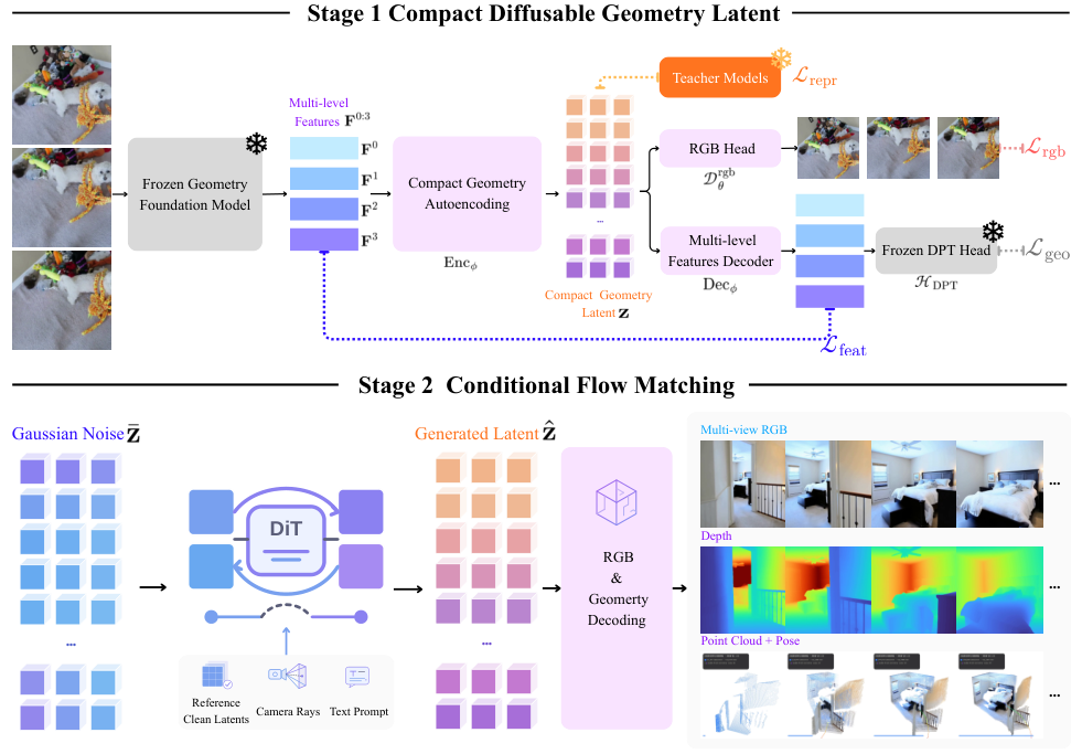
A detail the diagram does not show, and the code does: DA3's encoder emits a CLS
token alongside the patch tokens, and the codec does not encode it. GAE.encode
slices it off (fv[:, 1:, :]), and on the way back _format_recon_for_dpt hands
the frozen head a tensor of zeros in the CLS slot. So the head is being fed
a feature hierarchy that is structurally correct and globally lobotomised, and
still reads metric depth and cameras out of it. That is either a strong statement
about how little the DPT head uses its CLS token or a quiet source of the error
in the tables below; the paper does not say which, and it would take one ablation
to find out.
The two decoders are not twins
The parameter census is the other half of the "native" story, and it cuts both ways.
GAE-D64-1B is a 0.93B flow transformer on top of 2.56B parameters that are frozen while it trains, of which 2.11B come from two models GAE never trains at all. The learned geometry decoder has zero weights: geometry is read by Depth Anything 3's own DPT head. The learned RGB head has 203.2M, which is 45% of every trained weight in the codec.
| module | role | parameters | trained by GAE |
|---|---|---|---|
| DA3-GIANT-1.1 | encoder + DPT geometry head | 1,355,674,125 | no — frozen at both ends |
| codec.enc_* | fused 12288-ch tensor to z | 126,132,352 | yes |
| codec.dec_proj/dec_attn | shared decoder trunk | 50,453,504 | yes |
| codec.dec_conv | trunk to 4 x 3072 features | 73,509,888 | yes |
| codec.rgb_head | trunk to pixels | 203,215,436 | yes |
| codec.repa_proj | C-RADIO projector, training-only | 1,231,104 | yes, then unused |
| codec (other) | level statistics + level weights | 24,580 | no — buffers, plus 4 level weights |
| flow transformer | GAEFlowTemporal, 28x768 + 6x2048 | 933,675,138 | yes |
| Qwen3-0.6B | text encoder, cross-attention | 751,632,384 | no — frozen |
| total at inference | one frame end to end | 3,495,548,511 | 1.39B of it |
repa_proj is the projector for L_tok, which the paper says is discarded after codec training; it is still in the shipped checkpoint, and gae/pipeline.py filters it out of the missing-keys check when loading. Every GAE tensor in the repo is F32, as is DA3-GIANT-1.1.
Reading that column: the learned geometry decoder has zero parameters. Geometry is read by a head GAE never trains. The learned RGB decoder has 203,215,436 — 45% of every trained weight in the codec, and more than the encoder and the feature decoder put together. Appearance is the expensive, learned readout here. Geometry is the one that was already there.
Which is the point, and also the risk. Nothing in the architecture stops the codec from spending its bottleneck on whatever makes the 203M-parameter RGB head happy, because that is where the gradient pressure is. The counterweight is that the geometry head is frozen, so the feature reconstruction has to stay legible to the original DA3 interface — the paper is explicit that this "prevents the decoder from adapting around information lost during compression."
There is a second asymmetry, and it is in the training config rather than the
paper. From configs/gae_64.yaml:
# RGB-only latent jitter: perturb latents before RGB decode so the head is
# robust to noisy diffusion-generated latents (feature/REPA/geo decode clean z).
rgb_latent_jitter_mode: mixed
rgb_latent_jitter_sigma: 0.1
rgb_latent_jitter_prob: 0.7
rgb_latent_jitter_start_step: 30000
From step 30,000, 70% of codec training steps decode RGB from a perturbed latent while the feature and geometry branches decode the clean one. The RGB head was deliberately hardened against the imperfect latents Stage 2 emits at sample time. The geometry branch was not. If that matters, it should show up as a bigger degradation on the geometry side when you swap encoded latents for sampled ones — and the paper measures exactly that, in two tables that share a codec.
It does show up. Every geometry metric degrades by a third to two thirds when the latent comes from the flow model instead of from real frames. I cannot attribute that to the jitter asymmetry on this evidence — a sampled latent is off distribution in more ways than Gaussian noise at sigma 0.1 — but it is the cheapest experiment in this article: re-train the codec with the jitter applied to both branches and see whether the gap narrows.
The row that survives is the camera track. Sampled geometry recovers the trajectory to an ATE of 0.010 against the dataset cameras, where Pi3 reading the real target frames scores 0.009. The generated world's cameras are as recoverable as a real scene's, which is a stronger statement than any of the depth numbers.
Does the choice of latent actually matter
The paper's argument is a controlled swap, and it is the right experiment: seven latents dropped into the same DDT-style flow model with the same camera conditioning, the same budget, the same sampler — nine views at 252×252 from one reference, 50 Euler steps, CFG 2. Only the encoder, the decoder, and the input and output projections forced by the latent shape change.
The abstract's headline — FVD down 12.7% on RealEstate10K and 23.1% on DL3DV — is GAE-64 against SD-VAE, which is genuinely the strongest competing latent on both datasets. Against the geometry-native thing GAE was distilled from, raw DA3 level 0, the margins are 24.4% and 23.8%. And the VGGT column is the one that answers "is this just prettier frames": trajectory error 0.0034 against SD-VAE's 0.0072, which is the "halved" in the abstract, measured by a reconstructor that shares no backbone with any latent in the table.
Two things keep this honest and are worth repeating because most coverage will not. Raw DA3 L3 is a geometry-native latent that loses to a pixel VAE by a mile — so "geometry-native" is not sufficient on its own, and the conditioning work is not decoration. And the two faded rows are complete external systems rather than latents in the shared harness; the paper greys them out of its own ranking and says why, which is the correct call and also leaves Gen3R's 25.7 FID on RealEstate10K sitting right there in the table — a dead heat with GAE-128's 25.6, and 1.4 ahead of GAE-64's 27.1.
Then there is the part that makes this article's subject legible as a research question rather than a slogan. The paper evaluates its geometry twice, under two protocols it names separately:
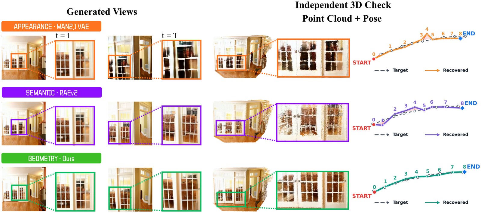
- Post-hoc. Run VGGT, MEt3R and a DA3 cross-check on the generated RGB. That is the lifted path — geometry estimated from pictures — and it is the right independent check precisely because it does not trust the model's own readout.
- Native. Decode depth, rays and point maps straight from the sampled latent and score them against Pi3 on the real target frames and against the dataset cameras. The appendix says the reason in one sentence: this "separates native geometry readout from the post-hoc RGB reconstruction used for the consistency table," and the common reference "avoids evaluating each method against geometry estimated from its own generated images."
A method whose only 3D evidence was its own decoder marking its own homework would deserve the suspicion it got. This one reports both — and the point clouds in the independent-check figure below are the lifted ones, VGGT run on everyone's frames including its own.
Three checkpoints, and which one you are looking at
This is where a reader gets misled if nobody says it plainly, because the paper's numbers, the project page's videos, and the released weights are three different models.
- The controlled model. Nine views at 252×252, trained on an equal mixture of RealEstate10K and DL3DV, eight GPUs, 0.93B flow transformer. Every generation number above — Tables 5, 6 and 7, the whole bake-off chart, and the filled dots in the reconstruction-to-generation chart — comes from this one. It is the model that argues. (Tables 1–4, including the hollow dots, depend only on the codec.)
- The final model. 81 views at 672×378, one to four prefix references, a multi-domain mixture adding ScanNet++, MVS-Synth, SpatialVID, OmniWorld and "several internally curated datasets," trained on 80 GPUs. The paper is unusually direct about its status: these results "are qualitative and are not part of the comparison." Everything you see moving on the project page, and both clips in this article, is this model.
- The released weights.
flow_gae64.pt, which the repo's README calls "a stronger continued-training model — larger resolution, more frames, and more training data," and then says the eval scripts "will not reproduce the exact paper numbers on these weights; they are expected to match or exceed them. Reproducing Tables 5–7 verbatim requires the original research checkpoint, which is not part of this release."
So: the thing you can download cannot reproduce the thing that was measured, and
the thing you can watch was never measured. Both of those are normal in this
corner of the field and neither is hidden — the README flags it under a heading
that starts "read before comparing to the paper," which is more than most
releases do. The codec is the exception and the README says so: Tables 1–4
depend only on gae_{64,128}.pt, which is what shipped, so the latent
diagnostics and the reconstruction numbers track directly.
What actually ships
- task
- image-to-video
- library
- pytorch
- safetensors
- 2 shards
- largest file
- 3.74 GB
- files
- 14
- downloads
- 0
- likes
- 3
Thirteen files, and two copies of the model: gae_64.pt and codec/model.safetensors are the same 454.6M-parameter codec, flow_gae64.pt and transformer/diffusion_pytorch_model.safetensors the same 933.7M-parameter flow model, so half the bytes are a second copy in another container. Both safetensors files are F32. GAE-128 is in the configs and not on the Hub.
repo last modified 2026-09-22
Weights are released, and the release is more complete than most: training code
for both stages, the eval scripts that produce each table, the dataset packers,
a Gradio app, and a run_demo.sh that builds a venv and downloads checkpoints.
The parts that are not GAE's to give are named rather than vendored — DA3-GIANT
comes from depth-anything/DA3-GIANT-1.1 on first use, text from
Qwen3-0.6B, and the external
evaluators — VGGT and
Pi3 — are --vggt-ckpt / --pi3-ckpt
arguments you supply.
Three things to know before planning anything around it.
The licence is academic-use only. Tencent's terms grant the usual MIT-shaped
permissions and then add one bullet that removes most of them: "You agree to use
[it] only for academic purposes, and refrain from using it for any non-academic,
commercial or production purposes under any circumstances." The frozen backbone
is separately CC BY-NC 4.0. There is no commercial path here, and the Hub card
carries no licence tag at all, so the only place that says so is LICENSE.txt.
"1B" is the flow transformer, not the system. The paper says so — the 0.93B figure "covers the trainable Stage 2 generator and excludes the frozen DA3 encoder, space–time codec, and text encoder." Count everything a forward pass touches and it is 3.50B parameters. GAE trained 1.39B of them; the other 2.11B are DA3-GIANT and Qwen3-0.6B, frozen and not yours to change. At the shipped F32 that is about 14 GB of weights before a single activation.
GAE-128 is not released. It is the variant that wins reconstruction (Table 3: PSNR 28.76 single-view against GAE-64's 27.30) and the better Chamfer and point-map numbers on generated RealEstate10K geometry (Table 7: 0.432 and 0.813 against 0.501 and 0.924). The configs are in the repo, the checkpoint is not.
Text to image, and the honest limit of a native readout
The same flow checkpoint does text-to-image, because T2I is co-trained inside the
video model rather than bolted on — cotrain_t2i.every_k: 4 interleaves a
single-view batch every four multi-view updates. The ablation says this is not a
free extra: turning T2I co-training off takes RealEstate10K FVD from 225.7 to
472.9, the largest single effect in Table 8. Single images are what teaches
this model what the world looks like; the video data teaches it how the world
moves.
Every generated image comes with depth and a point cloud from the same latent,
and generate_t2i.py writes the .ply by default.
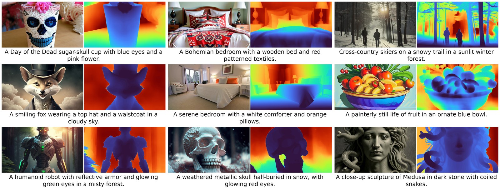
That figure is the best argument for reading the depth maps rather than the images, and it sorts cleanly by prompt. The two bedrooms and the snowy forest trail are scenes, and their geometry is doing real work: floors and the trail recede through several bands, tree trunks sit at visibly different distances, furniture separates from walls. This is roughly what DA3 would read off a photograph of the same room. The sugar-skull cup and the painted fruit bowl are objects on a surface, and they get relief on the subject over a flat wash behind it. The fox in a top hat and the humanoid robot are portraits, and they get a silhouette: hat, ears, muzzle and shoulders all at one depth, cut out of a uniform background.
Which makes sense. The video half of the training mixture is scenes with parallax. The single-image half is BLIP3o, JourneyDB, ImageNet and friends, where nothing ever moves and the only geometric supervision available is whatever the frozen DA3 head reads off the image — and on a Midjourney-styled portrait with a bokeh background, that is not much. A native geometry readout is useful precisely because it tells you what the model believes about 3D rather than what a reconstructor can talk itself into. On "a smiling fox wearing a top hat," it believes the fox is a sticker.
The paper says as much, in its own register: these examples "demonstrate capability rather than benchmark text-to-image quality." That is the right claim and it is smaller than the demo looks.
What I'd want measured
Sorting this article's claims by what they rest on. Reported is every
benchmark number, all of it from the paper's Tables 1–8 and the repo's README.
Measured is the parameter counts, read tensor by tensor out of the shipped
safetensors headers over HTTP; the latent element counts; the forward path traced
through gae/pipeline.py, src/stage1/gae_codec.py and
scripts/eval/eval_generation.py at a61ebe5; the config values quoted verbatim;
and the time-shift arithmetic. Reasoned is the reading of why the two
decoders are asymmetric, the suggestion that the jitter schedule explains the
reconstruction-to-generation gap, and the claim about what the T2I depth maps
show. Those are below with the experiment that would kill each.
What would change my mind
6 claims above, and what would falsify each
The point clouds are native. The geometry decode path reads only the sampled latent and never the decoded RGB; deleting the RGB head would leave the cloud's coordinates unchanged.
This is the one that matters, and it is a graph property, so it is cheap to check. In
scripts/eval/eval_generation.py,_recover_view_pointcloudsbuilds coordinates asray[..., 3:] + depth * ray[..., :3]and usesrgb_imgsonly to fill thecolsarray;GAE.decode_geometry(z, H, W)takes no RGB argument andGAECodec.decode/decode_rgbare siblings off_decode_trunk(z). To falsify it: run the demo with the RGB head's weights randomised and diff the exported.plycoordinates against a normal run. If any coordinate moves, there is a path I did not find — the two places to look are thegeo_adapterbranch indecode_geo, which the released config leaves unconfigured (so it is the identity) and which the public pipeline never calls, and the autoregressive rollout, which decodes RGB per chunk and hands it to the same builder before the chunks are overlap-aligned. If they are bit-identical, this claim holds for the released checkpoint and nothing else.The RGB head is trained to survive sampled latents and the geometry branch is not, and that asymmetry is part of why generated geometry degrades 30–65% against the same codec run on real frames.
The first half is config, not inference:
rgb_latent_jitter_sigma: 0.1atprob: 0.7from step 30,000, applied only before the RGB decode. The second half is a guess. Train two GAE-64 codecs to the same step count, one with jitter on the RGB branch only and one with it on both, freeze each, train matched flow models, and compare Table 4 against Table 7 for each. If the gap is the same either way, sampled latents are off distribution in ways Gaussian jitter does not model and this explanation is worthless — which is my own prior at maybe 50/50.Zeroing DA3's CLS token costs the frozen DPT head real accuracy.
GAE.encodedrops the CLS token and_format_recon_for_dptsubstitutes zeros, so the head never sees it. Nobody has published what that costs. Take real frames, run DA3 normally, then run it again with the CLS token zeroed at every level, and compare AbsRel, δ₁ and the recovered trajectory. If the difference is in the third decimal, the CLS token is decorative for dense prediction and this is a non-issue; if depth degrades measurably, then part of GAE's Table 4 gap is a plumbing decision rather than a compression limit, and encoding the CLS token would be a cheap win.'Geometry-native' is not sufficient on its own — the conditioning work is what makes the latent generate well, and raw DA3 L3 losing to a pixel VAE is the proof.
Table 5: raw DA3-GIANT L3 posts FVD 488.9 on RealEstate10K against SD-VAE's 258.6, in the same harness. To overturn this you would have to show the L3 baseline was crippled by something other than its own conditioning — an input/output projection that cannot absorb 3,072 channels, a learning rate tuned for 64-channel latents, a time-shift schedule derived for a much smaller state. The paper holds the flow architecture and schedule fixed on purpose, which is exactly what makes a 3,072-channel latent's projections a plausible confound. Re-run L3 with a per-latent learning-rate and shift sweep; if it closes on SD-VAE, the conditioning story is weaker than the table makes it look.
GAE-D64-1B is 3.50B parameters at inference, of which 2.11B are frozen; the '1B' is the flow transformer alone.
Counted from the safetensors headers: 933,675,138 in the flow transformer, 454,566,864 in the codec, 1,355,674,125 in DA3-GIANT-1.1 and 751,632,384 in Qwen3-0.6B. The paper agrees about what its own figure covers. The soft spot is the text encoder — if the released inference path loads a quantised or truncated Qwen3, or only its first N layers, my total is high by up to 0.75B. Print the state dicts after
GAE.from_pretrainedplus the text encoder and settle it in one line.Native geometry from a text prompt degrades with how subject-centric the prompt is: real layered structure for scenes, relief-on-a-flat-wash for objects, a silhouette for portraits.
This is read off nine examples in one figure, which is thin. Generate a few hundred images across a prompt taxonomy — portrait, object on a surface, interior, landscape, street — decode depth from each latent, and measure the within-subject depth variance against the subject-to-background step. If portrait prompts turn out to have as much internal relief as interiors, I am pattern-matching on a curated figure. The stronger version of this test compares GAE's decoded depth against DA3 run on GAE's own output image: if they agree closely everywhere, the native readout is adding nothing over the lifted one for T2I, which would be the most interesting negative result available here.