2026-09-10 · 32 min · depth-estimation · diffusion-transformers · monocular-depth · lora · quantization · computer-vision
Marigold V1 turned a ~1B-parameter Stable Diffusion U-Net into a monocular depth estimator by fine-tuning it on 74,000 synthetic images, and it became one of the most-cited "repurpose a generative prior" tricks in the field. Marigold V2 claims the same trick, the same name, and the same "cheap to fine-tune" pitch. It is not the same model. V2 is a rank-128 LoRA on top of Qwen-Image-Edit-2509, a 20.43-billion-parameter diffusion transformer, quantized to 4-bit before anything gets trained. The recipe carried over — repurpose a generative prior into a dense predictor. The model and the cost did not.
- task
- depth-estimation
- license
- apache-2.0
- safetensors
- 9 shards
- largest file
- 1.85 GB
- files
- 30
- downloads
- 0
- likes
- 22
- languages
- en
This repo holds LoRA adapters, not a full model — its own parameter count is not directly comparable to the backbone it adapts. The 17.25 GB repo size below is the number I use throughout this piece to cross-check the checkpoint-by-checkpoint byte accounting.
repo last modified 2026-09-09
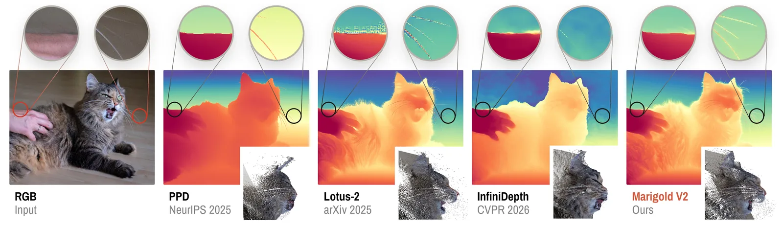
The name is doing a lot of work
Here is the comparison that matters, and it is checkable without running anything — Hugging Face's own model metadata reports parameter counts per subfolder of a repo.
Marigold V1's backbone is Stable Diffusion 2's U-Net:
prs-eth/marigold-depth-v1-0/unet/diffusion_pytorch_model.safetensors
  → 3,463,772,592 bytes at fp32 → 865,943,148 parameters
Qwen-Image-Edit-2509's DiT (the part Marigold V2 actually fine-tunes):
Qwen/Qwen-Image-Edit-2509/transformer/diffusion_pytorch_model.safetensors.index.json
  → metadata.total_size = 40,860,802,176 bytes at bf16 → 20,430,401,088 parameters
That is a 23.6× jump in backbone size, and it is not incidental — a 60-layer,
3072-dim, 24-head diffusion transformer (num_layers: 60, attention_head_dim: 128,
per the transformer's own config.json) is qualitatively a different kind of
object to fine-tune than a convolutional U-Net, which is exactly why the paper's
actual title is "Revisiting Diffusion Transformers for Monocular Depth
Estimation," not "Marigold V2." The pipeline this transformer sits in — Qwen2.5-VL-7B
text encoder (8.29B params by weight bytes; released only in the "Plus" edit
variant used here) plus a small VAE — totals 57.7 GB on disk; the text encoder
is never loaded at Marigold V2 inference time (more on that below), and the VAE
is the only part of Qwen-Image-Edit-2509 that gets touched besides the DiT.
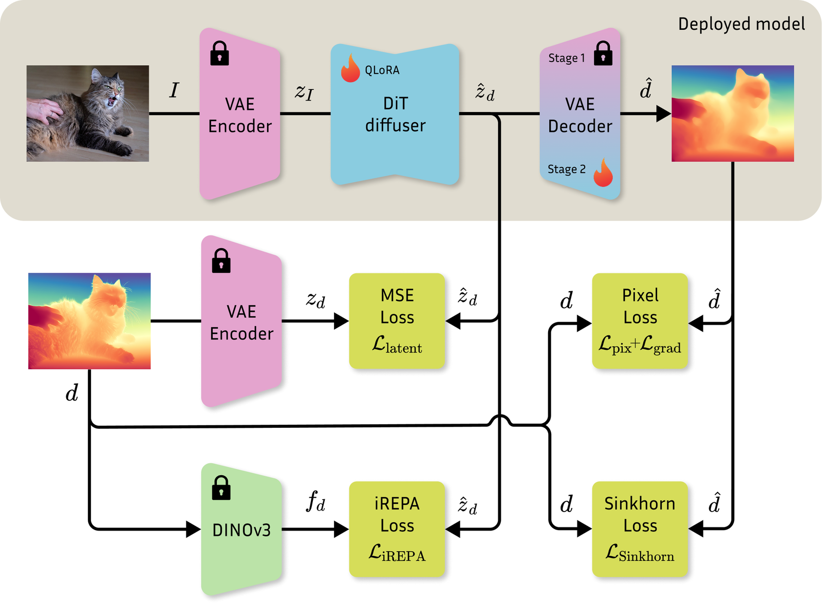
What actually gets trained is much smaller than either backbone — a rank-128 QLoRA adapter, 851,779,584 parameters, verified later in this piece by reading the checkpoint files' own tensor headers. That is roughly the same parameter count as the whole of Marigold V1's U-Net, just spent very differently: as a thin adapter riding on a 20B-parameter frozen transformer instead of as the entire trainable model.
Four models, one idea
Marigold V2 is the fourth release under this name, and the project's own "Marigold Lineage" section is honest about what changed each time:
- Marigold (CVPR 2024, arXiv 2312.02145) — fine-tuned Stable Diffusion's U-Net on synthetic data, a few GPU-days.
- Marigold Computer Vision / V1.1 (TPAMI 2025) — extended to normals and intrinsic decomposition, fewer sampling steps, moved to
diffusers. - Marigold-DC (ICCV 2025) — turned sparse depth completion into test-time guidance, no retraining.
- Marigold V2 (this paper) — swaps the U-Net for a diffusion transformer, full fine-tuning for 4-bit QLoRA, a multi-step denoising schedule for one fixed-timestep pass, and adds SinkLoss + iREPA for detail.
Every step kept the founding bet — a pretrained image generator already encodes a useful prior about scene geometry, so start from it instead of training a depth network from scratch — while quietly swapping out everything underneath it. V2 is the biggest swap of the four.
One forward pass, not a denoising loop
The efficiency claim that is real: Marigold V2 does not run a multi-step diffusion sampler at inference. Given an RGB image and its VAE-encoded latent , the DiT is conditioned on and a fixed timestep , and trained to directly regress the velocity between the RGB latent and the target (depth/normals/albedo) latent :
Because is fixed, the rectified-flow objective collapses to a direct latent regression — there is no trajectory to integrate. At inference this is one subtraction:
That single forward pass is implemented literally as a fixed constant in the
released code, not a scheduler configured to run one step — scripts/infer.py
never touches a scheduler at all:
# marigoldv2/experiments/20260316_qwen_depth/network_graph.py
# Fixed timestep t = 0.499, computed in bf16 exactly as during training.
timestep = torch.full((B,), 499.0, device=device, dtype=run_dtype) / 1000.0
...
model_pred = diffuser(**call_kwargs, return_dict=False)[0]
...
if self.predict_vel:
    latents = model_input.to(vae.dtype) - model_pred.to(vae.dtype)
(499/1000 rather than an exact 0.5 — presumably a scheduler discretization
artifact from however the training config resolves t=0.5 into a bf16
timestep embedding; the paper's math uses throughout and the
difference is immaterial to the result.)
Quantize, then adapt: the QLoRA setup
The DiT is loaded once, quantized to NF4 4-bit via bitsandbytes, and a
rank-128 LoRA adapter is attached to a fixed list of module name patterns.
This is the entire component loader, trimmed to the load-bearing lines:
# marigoldv2/experiments/20260316_qwen_depth/component_loader.py
quantization_config = DiffusersBitsAndBytesConfig(
    load_in_4bit=True,
    bnb_4bit_quant_type="nf4",
    bnb_4bit_compute_dtype=torch.bfloat16,
    llm_int8_skip_modules=skip_modules,   # ["transformer_blocks.0.img_mod"]
)
transformer = QwenImageTransformer2DModel.from_pretrained(
    model_id, subfolder="transformer", torch_dtype=torch.bfloat16,
    quantization_config=quantization_config,
)
transformer = prepare_model_for_kbit_training(transformer, use_gradient_checkpointing=False)
transformer.requires_grad_(False)
_dequantize_modules_to_bf16(transformer, dequantize_modules)  # ["proj_out"]

lconf = LoraConfig(
    r=128, lora_alpha=128, lora_dropout=0.0, init_lora_weights="gaussian",
    target_modules=[t for t in lora_cfg_in.target_modules if "proj_out" not in t],
)
transformer.add_adapter(lconf)
for name, p in transformer.named_parameters():
    if "lora_" in name:
        p.requires_grad_(True)
Two details are easy to miss and both matter: the very first block's
modulation layer (transformer_blocks.0.img_mod) is skipped during
quantization — kept at full precision, presumably because errors there
propagate through all 60 blocks — and the final output projection
(proj_out) is dequantized to bf16 and fully excluded from LoRA, trained
at full precision if trained at all, rather than adapted through a low-rank
update. Everything else — 21 named module patterns per block, repeated across
60 transformer blocks, plus three global modules (img_in, txt_in,
norm_out.linear) — gets the rank-128 treatment. I verify the exact resulting
parameter count later in this piece by reading the checkpoint files directly,
rather than trusting the config.
iREPA: aligning to the target, not the input
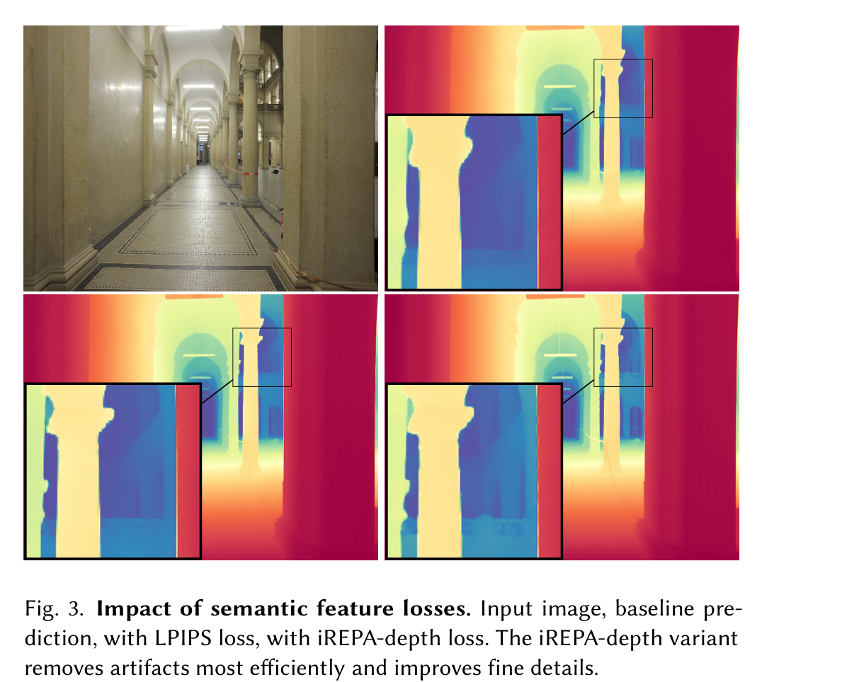
Pixel losses ( on the decoded prediction, on its spatial gradients) push the model toward the right value at each location, but they say nothing about whether the structure of a cluttered region — foliage, a patterned railing, a head of hair — survives. The paper's fix is iREPA, a representation-alignment loss with one deliberate twist. REPA (the technique it is named after) aligns a diffusion model's internal features to a frozen visual encoder's features of the input — DepthMaster does this with DINOv2 on the RGB image, and Pixel-Perfect Depth folds semantic features from vision foundation models into the diffusion process the same way. Marigold V2 instead aligns the DiT's internal features to a frozen DINOv3 encoder's features of the ground-truth depth map:
# marigoldv2/loss/loss.py — IREPADinoV3SpatialLoss
gt_in = self._to_dino_inputs(gt)            # gt = ground-truth depth/normals/albedo
with torch.no_grad():
    gt_out = self._feature_model(pixel_values=gt_in)   # frozen DINOv3-ViT-B/16
gt_tokens = self._extract_patch_tokens(gt_out)
...
# student_feature_keys point at captured DiT hidden states, not the prediction
feat = self._resolve_key(batch, k)          # out/qwen_dit_hidden_state_-1, _-8
...
l_tok = self._token_l1(s_tok, gt_tokens, token_mask)
l_pair = self._pairwise_structure_loss(s_tok, gt_tokens, token_mask)
The gt_key fed to DINOv3 is depth_rel_m11 — the normalized ground-truth
depth map, not the RGB input — and the "student" side is not even the decoded
prediction; the config asks for two of the DiT's own internal hidden states,
captured mid-forward-pass by QwenImageEdit2509Step:
# training_relative_log_depth_config.yaml
QwenImageEdit2509Step:
  kwargs: { capture_hidden_states: true, hidden_state_indices: [-1, -8] }
IREPADinoV3SpatialLoss:
  student_feature_keys: [out/qwen_dit_hidden_state_-1, out/qwen_dit_hidden_state_-8]
  student_feature_weights: [1.0, 0.7]
This is a real, defensible difference from plain REPA rather than a rebrand: the DiT already starts from an image-editing model, so it already has strong RGB-domain features — what it lacks is a push toward depth-domain structure, and that is exactly what aligning to DINOv3-on-the-target supplies. The paper's own ablation (Table 3) backs the choice: iREPA computed on RGB features helps over the no-iREPA baseline, but iREPA computed on the depth map itself helps more, on every one of the five zero-shot benchmarks.
SinkLoss: matching, not pointing
A plain loss forces the predicted value at pixel to equal the ground-truth value at that exact pixel. That is fine almost everywhere and actively wrong at object boundaries in synthetic training data — the paper shows why with a HyperSim crop: because HyperSim's ray tracer uses quasi-Monte-Carlo sampling, a pixel straddling a thin branch or a pane of glass is randomly assigned either the foreground or background depth, so no model can hit "perfect AbsRel" there and training against that noise just teaches the model to hedge — which is exactly what produces the blurry, flying-pixel halos around fine structure that every method in the comparison above suffers from to some degree.
SinkLoss relaxes the correspondence instead of tightening it. Tile the image into non-overlapping blocks; within each block, treat the 25 predicted values and the 25 ground-truth values as two point sets and find a soft one-to-one assignment between them by entropy-regularized optimal transport (Sinkhorn–Knopp), rather than pairing element with element by position:
where is the set of doubly-stochastic matrices with uniform marginals and is the Shannon entropy of the assignment. Intuitively: the loss only asks the network to produce the same multiset of depth values as the ground truth within a patch, up to a soft permutation — not the same value at the same coordinate. A prediction that gets the foreground and background values right but shifts the boundary by a pixel or two now pays almost no penalty, whereas a plain per-pixel loss would punish that boundary shift exactly as hard as getting the wrong depth entirely. That is the mechanism behind "fewer flying pixels, same fine detail": SinkLoss stops fighting the noisy ground truth at edges instead of trying to memorize it.
Invalid pixels get an elegant trick: any pair touching a masked-out pixel is
assigned a huge cost , so the optimal transport plan
matches invalid rows to invalid columns and leaves the valid entries with
clean marginals — no invalid ground-truth value ever supervises a valid
prediction. In code, this is WindowMatchedL1Loss, applied with weight 0
in Stage 1 and weight 1.0 in Stage 2:
# marigoldv2/loss/loss.py
cost_for_sinkhorn = real_cost * valid_pair + self.masked_cost * (1.0 - valid_pair)
log_K = -cost_for_sinkhorn / self.sinkhorn_tau        # τ = 0.1
log_M = _sinkhorn_log(log_K, n_iter=self.sinkhorn_iter)  # 5 iterations, log-domain
M = log_M.exp()
loss_pair = M * real_cost * valid_pair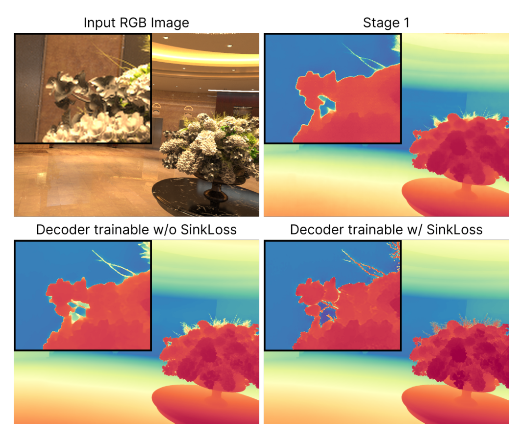
Three ways to compress depth into [-1, 1]
Before any of the above, metric depth has to be squeezed into the range the VAE encodes as a grayscale image. The paper ships, trains, and releases checkpoints for three different choices — an unusually complete ablation to actually ship as products rather than just a table row:
- Uniform — linear depth, Marigold V1's original choice.
- Disparity — linear in .
- Log — linear in , the paper's default.
Disparity (orange) is 1/D rescaled to [-1, 1]: it burns most of its output range on the first couple of meters, then goes almost flat — depth beyond ~5m gets barely any distinct encoder values, which is fine for close-up robotics but wastes the VAE's precision on a KITTI street scene. Uniform (gray) spends the range evenly in meters, so a 1cm error at 1m and a 1cm error at 19m cost the loss function the same, even though the second one is 19× less of a relative error. Log (teal) is the compromise the paper picks: because d(log D) = dD / D, an equal slice of the value range always corresponds to an equal relative change in depth — which is exactly what AbsRel measures. That is the derivation behind Eq. 11 in the paper: an L1 loss on log-depth is a first-order approximation of the AbsRel metric itself, so training on it and being scored on it point the same way.
Table 4's numbers back log clearly (average AbsRel / across the five benchmarks, all other settings held fixed): Uniform 5.04 / 97.10, Disparity 5.28 / 97.15, Log 4.72 / 97.71. The reason is a one-line derivation the paper gives and is worth spelling out: writing for the relative error that AbsRel measures,
An penalty on log-depth is, to first order, the same quantity as the AbsRel metric the model gets scored on. Training and evaluation stop fighting each other. Disparity, by contrast, is the opposite bet: it spends almost its entire output range on the first couple of meters (see the plot above) and goes nearly flat beyond that — good for foreground-focused tasks, bad for a KITTI street scene where most of the pixels are far away.
Two-stage training, mapped onto parameters
Nine checkpoints, verified byte by byte
huawei-bayerlab/marigold-v2-0 ships nine trainables.safetensors files,
and they come in exactly two sizes: 1,707,305,280 bytes and
1,853,909,694 bytes, a difference of 146,604,414 bytes. The model
card describes each checkpoint as "rank-128 LoRA adapters for the 4-bit
quantized DiT plus, where trained, the fine-tuned VAE decoder" — so the
prediction is that the larger files are exactly the ones with an unfrozen
decoder, and the size delta is exactly that decoder's weight.
A safetensors file's first 8 bytes are a little-endian u64 giving the
length of a JSON header that follows, listing every tensor's name, dtype,
and shape — no framework needed, just two HTTP range requests:
curl -r 0-7 "$URL" | # little-endian u64 → header length N
curl -r 8-$((7+N)) "$URL"  # the JSON tensor inventory itself
Doing this against one file of each size (depth/Log-stage1, 1,707,305,280
bytes, and depth/Log-stage2, 1,853,909,694 bytes) and summing tensor shapes
by dtype gives:
Log-stage1 (smaller) | Log-stage2 (larger) | |
|---|---|---|
Diffuser.*.lora_{A,B} (rank-128 adapter) | 851,779,584 params · 1,703,559,168 B | same |
iREPAStudentProjector.* (train-only DINOv3 head) | 884,736 params · 3,538,944 B | same |
VAE.decoder + VAE.post_quant_conv | — (not present) | 73,295,603 params · 146,591,206 B |
| header + data total (= file size) | 1,707,305,280 B | 1,853,909,694 B |
The delta between the two checkpoint sizes is 146,604,414 bytes; the VAE.*
tensor payload alone accounts for 146,591,206 of it, and the remaining
13,208 bytes is exactly the larger JSON header needed to describe 108 more
tensors — 146,591,206 + 13,208 = 146,604,414, to the byte. The model card's
"plus, where trained, the fine-tuned VAE decoder" claim holds exactly, and
depth/Log-stage1 and the six checkpoints ending in the larger size sort
into the two groups the training configs say they should. Rank-128 also
checks out analytically: img_in (128 × (64 + 3072) = 401,408), txt_in
(128 × (3584 + 3072) = 851,968), norm_out.linear (128 × (3072 + 6144) =
1,179,648), and 12 per-block module types at 786,432 or 1,966,080 params
each × 60 transformer blocks, sum to 851,779,584 exactly — the LoRA rank the
config declares and the LoRA parameter count the file actually contains are
the same number, derived two independent ways.
One more thing this check turns up: iREPAStudentProjector — the small
conv3x3 head that projects DiT hidden states into DINOv3's feature space
during iREPA training — ships inside every released checkpoint, at 3.5 MB
apiece. The evaluation code loads checkpoints by grouping tensors under their
top-level component name and only applying the ones matching a component
that actually exists in the inference config's registry
(marigoldv2/script/train/util.py, make_load_trainables_hook):
for name, module in registry["network_components"].items():
    if name in exclude_components or name not in by_comp:
        continue
    ...
    module.load_state_dict(by_comp[name], strict=False)
Inference configs only ever register VAE and Diffuser as network
components — there is no iREPAStudentProjector in evaluation/config/inference_depth.yaml,
because iREPA is a training-only loss. So that tensor group is silently
present in by_comp and silently never applied: harmless, but genuine dead
weight, roughly 31.9 MB spread across the nine checkpoints.
Putting the whole table together, with the file sizes as measured and the VAE-decoder column as verified above:
| Checkpoint | Output | Recipe | File size | VAE decoder |
|---|---|---|---|---|
depth/Log-stage2 (default) | affine-inv. log depth | Stage 1 (160k) → Stage 2 SinkLoss (30k) | 1,853,909,694 B | Yes |
depth/Log-stage1 | affine-inv. log depth | Stage 1 only, 160k steps | 1,707,305,280 B | No |
depth/Log-layered | see-through log depth | Log-stage1 + SinkLoss on LayeredDepth-Syn layer 8 | 1,853,909,694 B | Yes |
depth/Uniform-base | affine-inv. linear depth (V1-style) | Stage 1 recipe, 30k steps | 1,707,305,280 B | No |
depth/Disparity-base | affine-inv. inverse depth | Stage 1 + VAE decoder fine-tuning, 30k steps | 1,853,909,694 B | Yes |
depth/Disparity-layered | see-through inverse depth | Stage 1 recipe on LayeredDepth-Syn layer 8 | 1,853,909,694 B | Yes |
depth/Uniform-layered | see-through linear depth | LayeredDepth-Syn variant of Uniform-base (config not released) | 1,707,305,280 B | No |
normals | camera-space unit normals | angular + iREPA + SinkLoss, VAE decoder FT, 30k | 1,853,909,694 B | Yes |
albedo | linear RGB albedo, [0, 1] | + iREPA on ground-truth albedo, VAE decoder FT, 30k | 1,853,909,694 B | Yes |
Six checkpoints at the larger size, three at the smaller — matching the
brief's own accounting, and matching the ModelCard snapshot's repo-size
figure: 6 × 1,853,909,694 + 3 × 1,707,305,280 bytes of checkpoints, plus
~961 MB of text embeddings (next section) and the 47.8 MB paper PDF, sums to
almost exactly the 17.25 GB the Hub itself reports for this repo.
931 MB of text embeddings, most of it dead
qwen_text_embeddings/qwen_edit_2509_qwen_depth_realimg_prompt_embeds.pt is
931,153,857 bytes — 384× the size of its sibling
..._qwen_depth_prompt_embeds.pt (2,424,713 bytes) — with a
1,041,203-byte mask file alongside it. Qwen-Image-Edit-2509 replaces the text
encoder at both training and inference time with these precomputed
embeddings, so the 8.29B-parameter Qwen2.5-VL never has to load; the question
is what is actually stored in a file that large.
Torch's .pt format is a zip archive with a pickled data.pkl describing
tensor metadata and a data/0 file holding the raw storage — readable
without torch at all, since pickletools.dis will disassemble the
_rebuild_tensor_v2 call and its shape/stride arguments directly:
GLOBAL     'torch._utils _rebuild_tensor_v2'
GLOBAL     'torch BFloat16Storage'
BININT     465575936          # total storage elements
BININT1    0                  # storage offset
BININT1    8                  # shape[0]  ← 8 "context" slots
BININT2    16238              # shape[1]  ← sequence length
BININT2    3584               # shape[2]  ← Qwen2.5-VL hidden size
So the giant file is shape (8, 16238, 3584) in bf16, and the sibling
_realimg512_ file (19,384,278 bytes) that every training config and
scripts/infer.py actually points at is (8, 338, 3584) — same 8 slots, a
48× shorter sequence. Qwen2.5-VL is a vision-language model: a
sequence length in the thousands, for what the filename calls a "real image"
prompt, is patch tokens from an actual conditioning photo run through the VL
encoder once, concatenated with the instruction text — not per-training-image
prompts as I first guessed, but a handful of representative images encoded
at two different resolutions (the giant file is presumably the same 8
reference images at a much higher input resolution, hence far more visual
patch tokens; the "512" name matches the shorter sequence). , which is where the 384× comes from — not 384 distinct
prompts, one sequence-length blowup applied to the same 8 slots.
And here is the part that makes the giant file's size pointless rather than
merely large: every training and inference config in the repo hardcodes
effective_batch_size: 1 / max_train_batch_size: 1. The code that consumes
these embeddings resolves a batch mismatch like this:
# marigoldv2/experiments/20260316_qwen_depth/network_graph.py
@staticmethod
def _match_batch(t, B):
    if t.size(0) == B: return t
    if t.size(0) == 1 and B > 1: return t.expand(B, *t.shape[1:])
    if t.size(0) > B: return t[:B]          # ← this branch, always, since B is always 1
    ...
With batch size always 1 and 8 slots on disk, t[:B] takes slot 0 and only
slot 0, every single time this code runs, in training or in inference. The
other seven slots of every one of these embedding files — including 7/8 of
that 931 MB — are loaded into host memory by _torch_load_full and then
never read. It is not a bug (nothing crashes, nothing is wrong with the
output), but it is real, measurable waste: this repo ships roughly 815 MB of
a 931 MB file that no code path in the release ever touches. I also note
one small archaeological detail while reading the pickle headers: every one
of these .pt files' internal zip root is named
qwen_edit_2509_flux_depth_prompt_embeds, not ..._qwen_..._embeds — a
leftover from whatever earlier script (targeting FLUX, per the paper's own
backbone-transfer ablation in Table 5) first generated this embedding
format, unrelated to correctness but a real fingerprint of how the release
evolved.
The headline number, checked
The abstract's claim is "16–26% improvement in AbsRel over the previous best
on KITTI and ETH3D." Both numbers are real. Table 1 reports AbsRel after
aligning every method's prediction to ground truth with sklearn's
RANSACRegressor (1,000 trials, seed 42) fit in log space — the same
protocol Pixel-Perfect Depth uses, which the paper adopts explicitly so the
comparison is apples to apples:
# evaluation/depth/eval.py
_PPD_RANSAC = RANSACRegressor(max_trials=1000, random_state=_PPD_RANSAC_SEED)
_PPD_RANSAC_MODEL = make_pipeline(_PPD_POLY_FEATURES, _PPD_RANSAC)
...
_PPD_RANSAC_MODEL.fit(mask_pred[:, None], mask_gt[:, None])
This alignment removes the global scale/shift ambiguity every affine-invariant depth method has, and RANSAC (versus a plain least-squares fit) additionally discards outlier pixels before fitting — a materially more forgiving protocol than a naive fit, which is exactly why the paper follows PPD's exact procedure rather than inventing its own: a home-grown alignment would make the comparison meaningless.
| Dataset | Previous best (non-giant models) | Marigold V2 | Improvement |
|---|---|---|---|
| NYUv2 | Lotus-2 — 3.7 | 3.6 | 2.7% |
| KITTI | FE2E — 6.5 | 5.4 | 16.9% |
| ETH3D | FE2E — 3.8 | 2.8 | 26.3% |
| ScanNet | Lotus-2 — 4.0 | 3.7 | 7.5% |
| DIODE | FE2E — 5.6 | 5.2 | 7.1% |
("Non-giant" excludes DepthAnything V2, MoGe, MoGe-2, and — all trained on 5M+ images, gray-highlighted and excluded from ranking in the paper's own Table 1, since Marigold V2 trains on 74K.) The five-column average improvement is 12.1%, not 16–26%. The abstract's number is arithmetically correct — 16.9% and 26.3% are genuinely the KITTI and ETH3D deltas — but it quotes the best two of five columns as if they were representative; NYUv2's 2.7% gets no mention anywhere in the abstract or the website. Marigold V2 is the best model in its training-data class on every one of the five benchmarks, which is a real result — it just is not a uniform 16–26% better everywhere, and the paper's own prose is more careful about this than its abstract: Section 4.3 explicitly calls out ETH3D as the "especially strong" result rather than claiming the range applies broadly.
The pixels behind the numbers
AbsRel and do not directly measure "does fur look like fur" — the qualitative claim is a separate one, and the project website backs it with 249 real output images across six methods and fifteen scenes. Here are five of them, all six baselines and Marigold V2, real renders committed locally (no hotlinking):
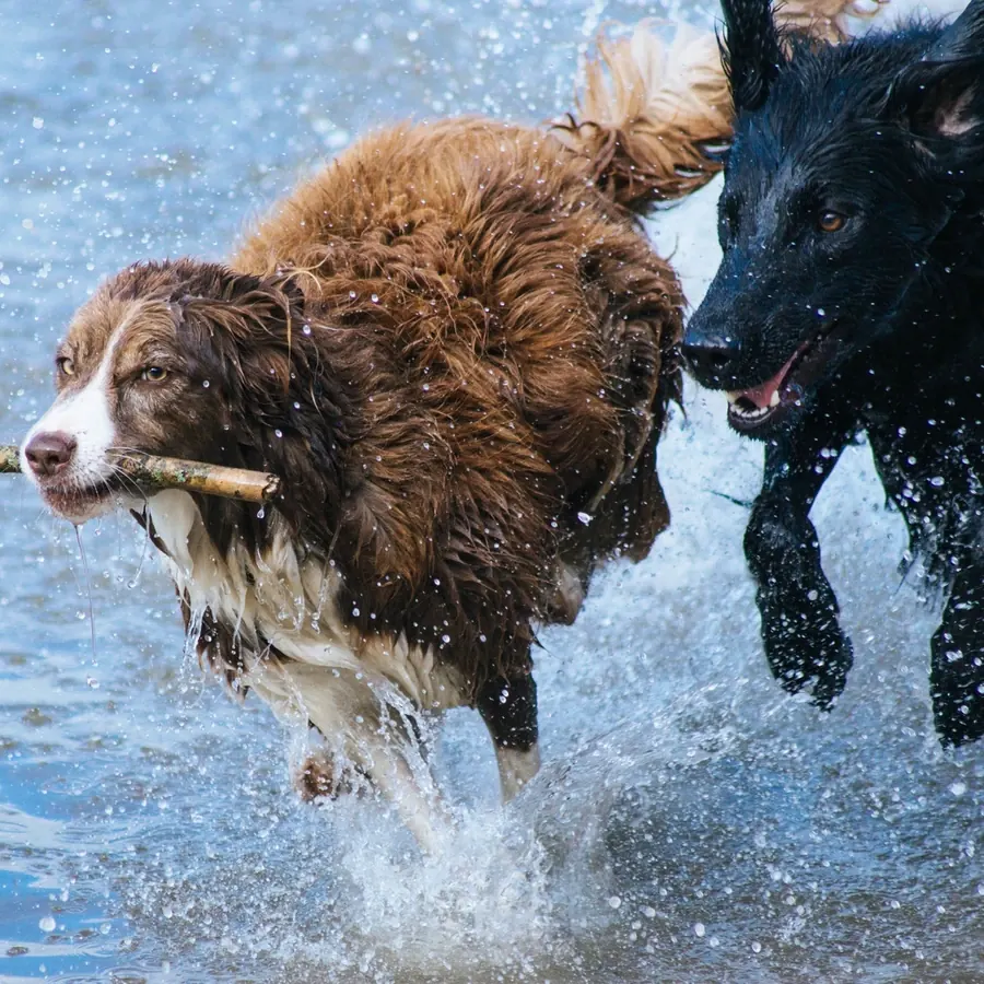



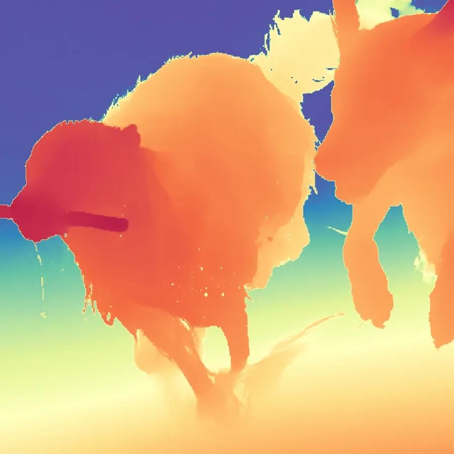
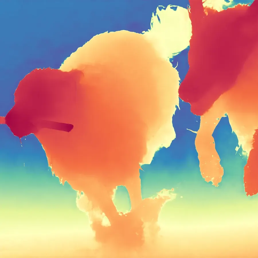























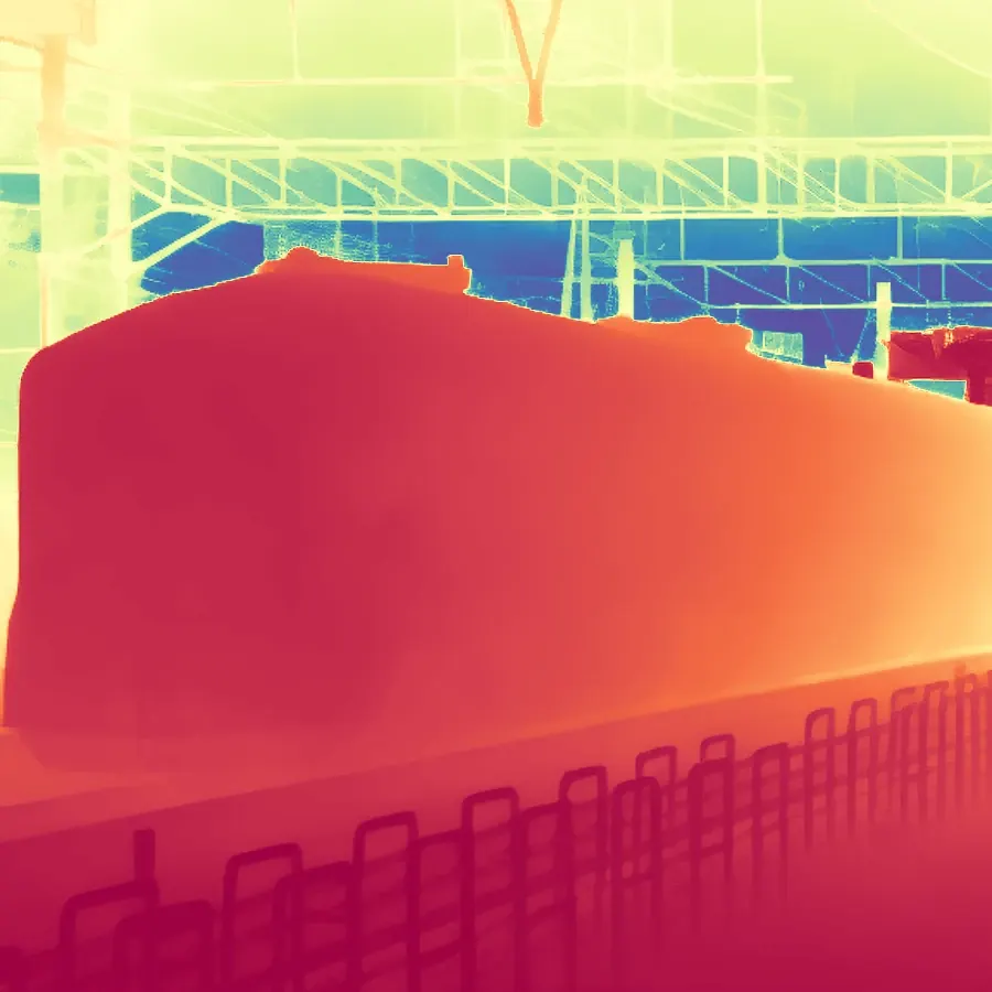

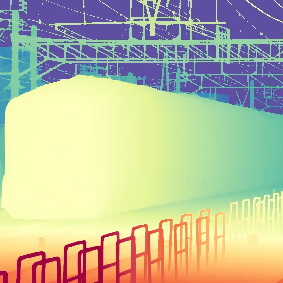
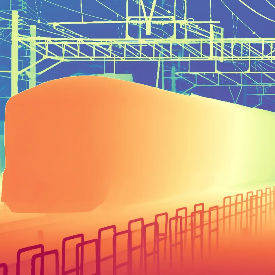
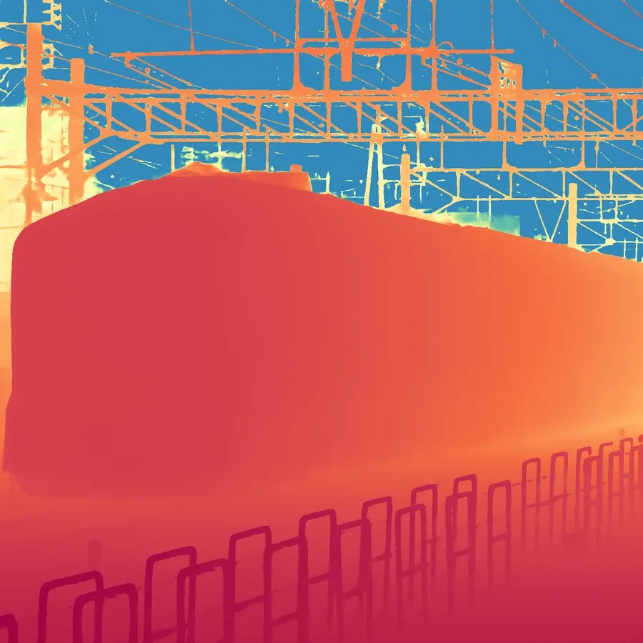
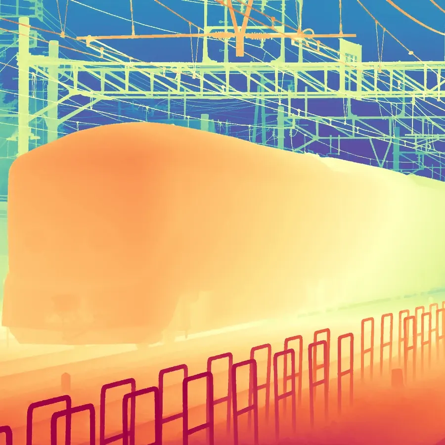
pick a scene, then flip the method row — look at the edges, not the color
What "cost-effective" is being measured against
The paper's own Table 6 latency/memory comparison is scoped to other diffusion-based depth estimators, measured on the same single 32 GB GPU:
| Model | 1024² latency | 1024² memory | 2048² latency | 2048² memory |
|---|---|---|---|---|
| InfiniDepth | 0.2 s | 1.9 GB | 1.2 s | 3.4 GB |
| PPD | 1.4 s | 5.6 GB | OOM | OOM |
| Lotus-2 (no sharpener) | 1.1 s | 26.1 GB | OOM | OOM |
| Lotus-2 | 8.9 s | 26.1 GB | OOM | OOM |
| FE2E | 3.9 s | 27.5 GB | OOM | OOM |
| Marigold V2 | 1.9 s | 16.9 GB | 9.6 s | 29.3 GB |
Inside this comparison set, Marigold V2's efficiency claim holds up well: it uses 35–39% less memory than Lotus-2 or FE2E and is the only method besides InfiniDepth that runs at all at 2048². "Single-step formulation avoids the iterative sampling... used by many diffusion models" (the paper's own phrasing) is a fair description of why.
What this table does not include is the comparison the brief for this
piece asked me to make: Depth Anything V2, the actual efficiency yardstick
for the field. DepthAnything V2 is a plain ViT, no VAE, no diffusion
transformer, no rectified-flow step, no 4-bit dequantization at inference —
just one forward pass through an encoder-decoder ViT. Its released sizes
range from 24.8M parameters (Small) to 335.3M (Large; no Giant checkpoint
was ever publicly released), confirmed directly from Hugging Face's
safetensors metadata for each. Even the largest public DepthAnything V2
checkpoint has roughly 1/61st the parameters of Marigold V2's frozen DiT
alone, before counting the LoRA, the VAE, or the fact that a 20B-parameter
transformer's 4-bit weights still have to sit in VRAM alongside activations
for every one of 60 transformer blocks. The paper never runs this comparison
because it is not a fair one architecturally — InfiniDepth, PPD, Lotus-2, and
FE2E are the right peer group for a "how expensive is the generative-prior
approach" question. But "cost-effective" and "cheap to run" in the abstract
and the model card, read without that scoping, invite exactly the comparison
the paper doesn't make: this is cheap relative to other diffusion-based
depth estimators, not cheap relative to the field's actual efficiency
frontier.
Does "less than a week on a consumer GPU" hold?
Yes, and the arithmetic is in the paper, not just the README. Stage 1 (the final model, not the ablations) runs 160,000 steps at batch size 1 and takes "slightly more than five days"; Stage 2 runs an additional 30,000 steps and takes "approximately one day" — both on the same single 32 GB GPU. Five-plus-one is six, which is under seven. Training mixes HyperSim at 768×512 (90% of batches) with vKITTI2 at 1216×352 (10%), and the entire claim rests on two choices working together: 4-bit quantization (so the frozen 20.43B-parameter DiT's weights fit in VRAM at all) and rank-128 LoRA (so only 851.8M parameters — 4.2% of the DiT — need gradients and an optimizer state). Neither the paper nor the code names the specific card — every mention is "a single 32 GB GPU" — which is itself worth flagging, since 32 GB is not a standard consumer VRAM size: NVIDIA's consumer line topped out at 24 GB (RTX 3090/4090) before the RTX 5090 shipped with exactly 32 GB in early 2025. I cannot verify which card was actually used — the repo never says — but the RTX 5090 is the only consumer GPU on the market that matches "32 GB" exactly, which makes "single consumer GPU" a plausible, specific claim rather than a vague one, if that is in fact the card.
Seeing through glass
Ordinary depth stops at whatever surface a ray first hits — for a window,
that is the glass, not the room beyond it. The see-through checkpoints
(Log-layered, Disparity-layered, Uniform-layered) are fine-tuned on
LayeredDepth-Syn (Wen et al. 2025, arXiv 2503.11633,
Princeton), a dataset that stores up to eight depth values per pixel
(depth_1.png through depth_8.png in the released
dataset) — one
for each surface a camera ray intersects as it passes through transparent or
reflective materials. Layer 1 is the ordinary first-surface depth every model
already predicts; layer 8 is the deepest recorded intersection, i.e.
whatever is furthest along that ray once every intervening pane of glass and
reflection has been passed through. Fine-tuning on layer 8 teaches the model
to report that, not the glass.
The paper's own numbers on the LayeredDepth-Syn validation split (Table 8) show why this needed a separate fine-tune rather than just relabeling the base model's output: the base depth model, evaluated on the same see-through ground truth, gets AbsRel 13.66 / 83.96; the see-through checkpoint gets 8.17 / 92.65 — nearly a 40% AbsRel reduction from training on the deeper layer specifically.
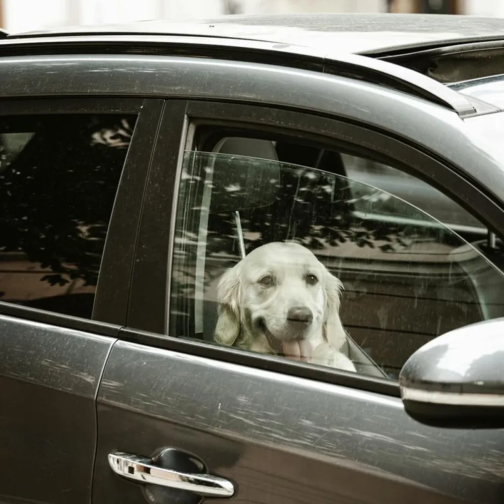


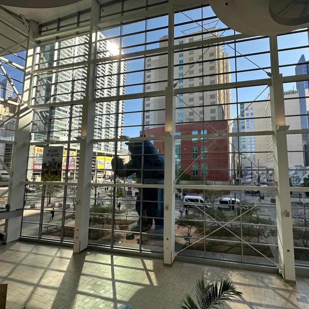





In the "Dog in a car" row, this is easy to read directly off the images: the regular-depth column renders the window as a flat, near-uniform surface — no dog visible at all behind the glass — while the see-through column recovers the dog's head as a distinct depth region behind the window pane. That is the model learning to look through the surface it used to stop at, not just a color remap.
Normals and albedo: same recipe, different supervision
The training framework is a small registry of losses and network-graph steps composed by YAML — swapping tasks means swapping the pixel-space supervision and the target the DINOv3 alignment runs on, not rewriting the pipeline. Surface normals replace the pixel loss with an angular loss and keep iREPA and SinkLoss; albedo drops SinkLoss and keeps + iREPA, both computed against ground-truth normals/albedo instead of depth.
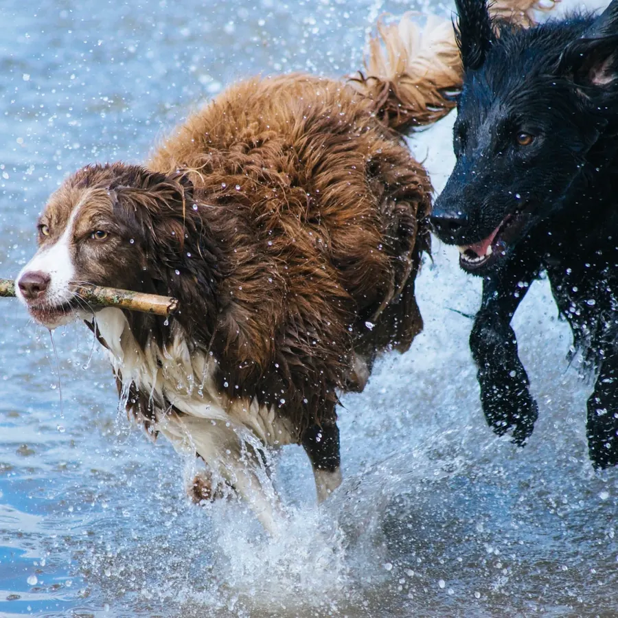
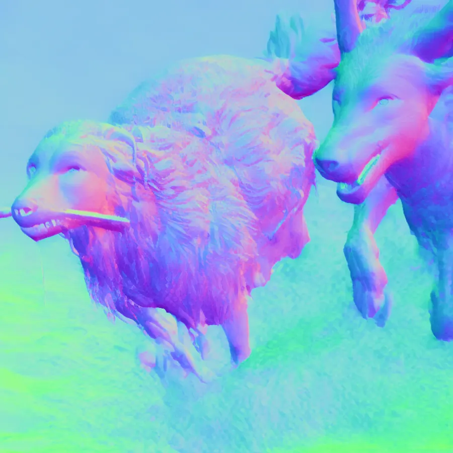

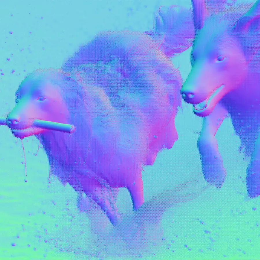
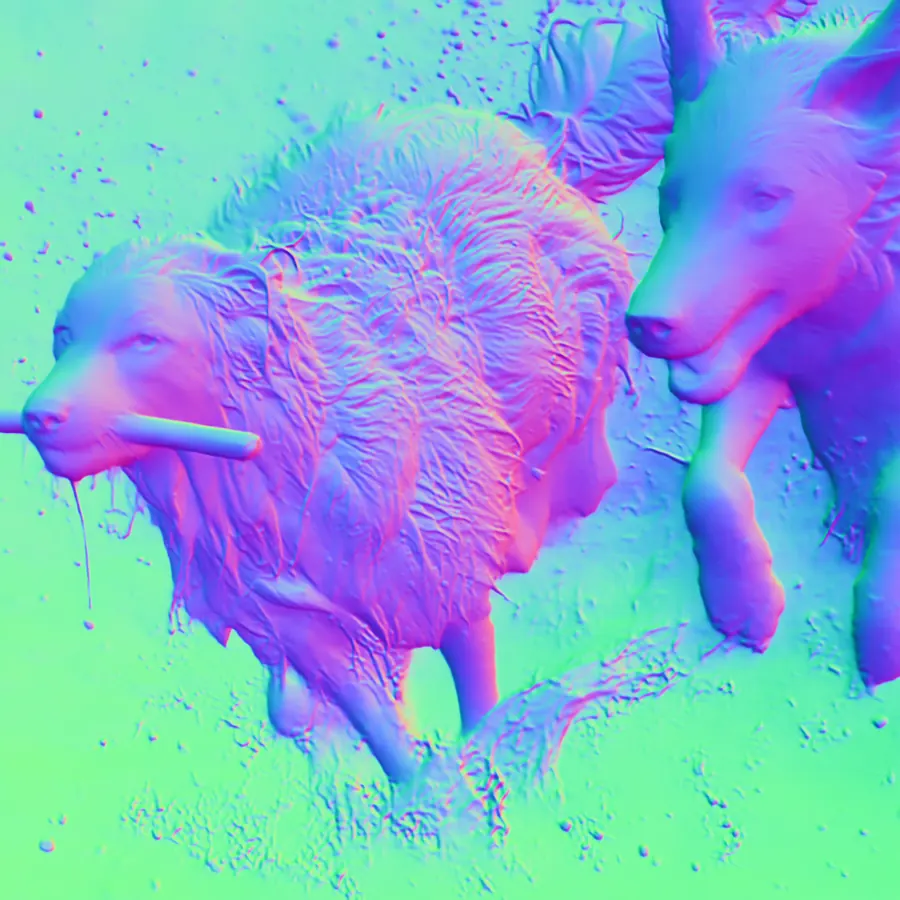

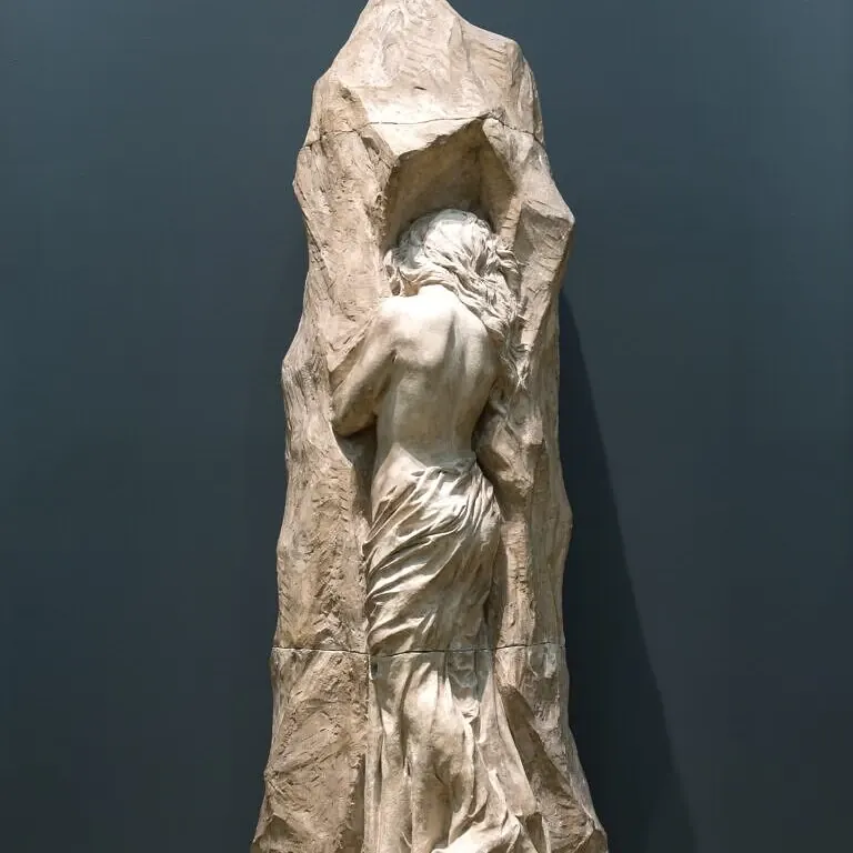






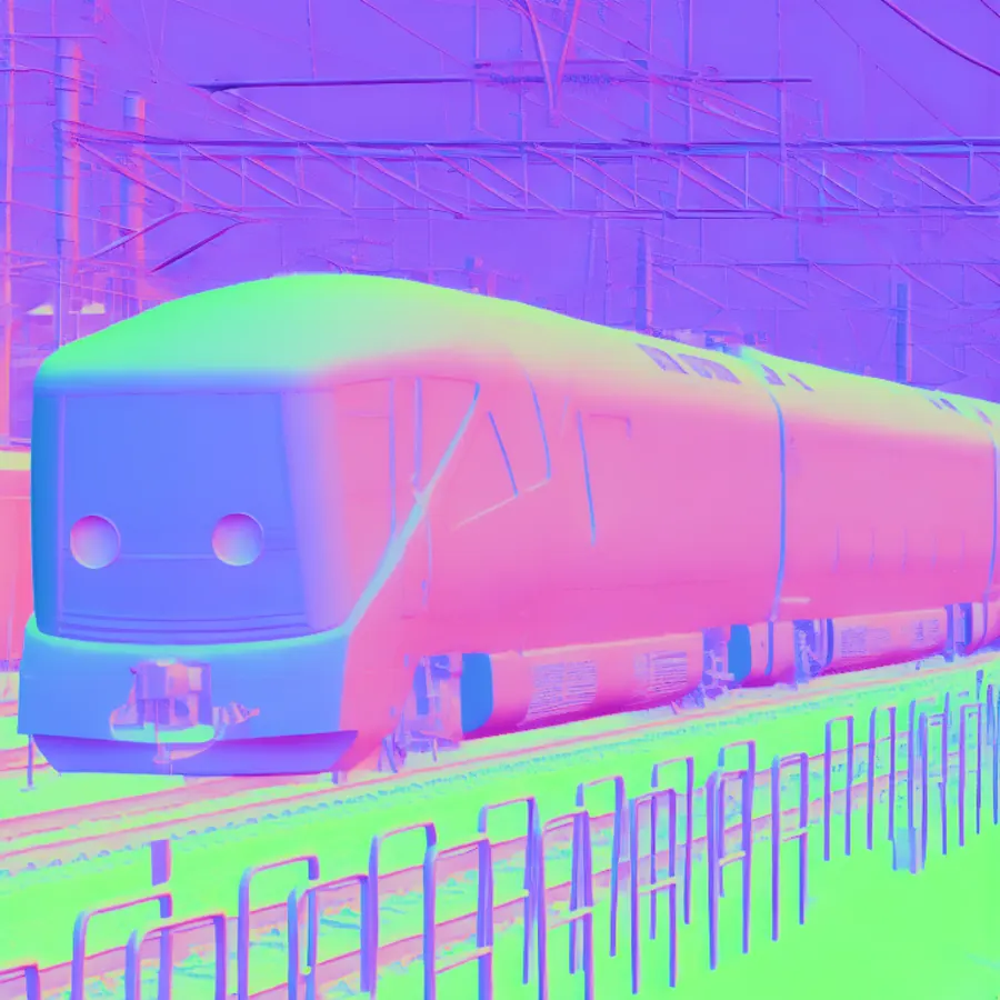
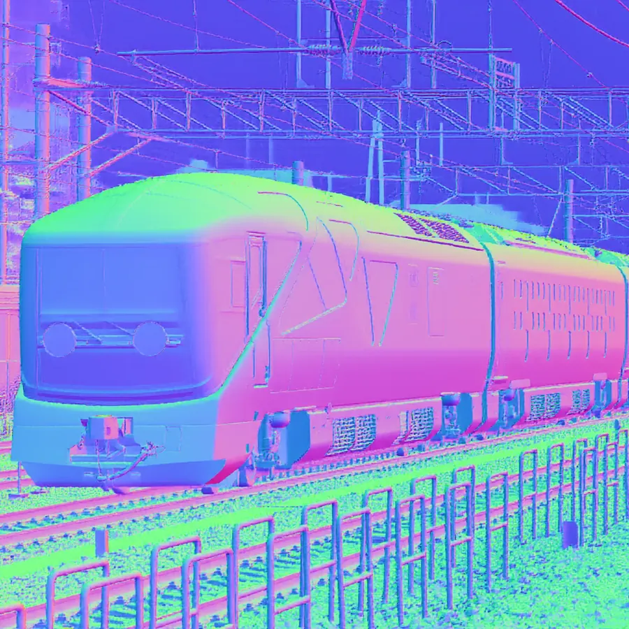
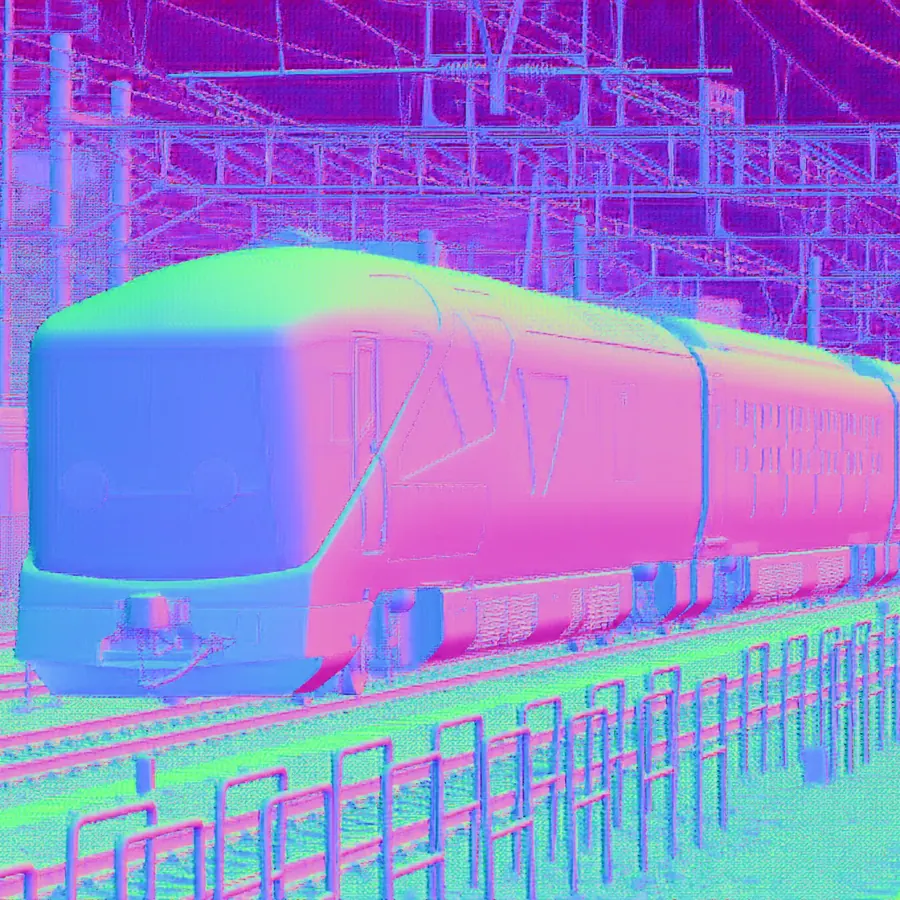
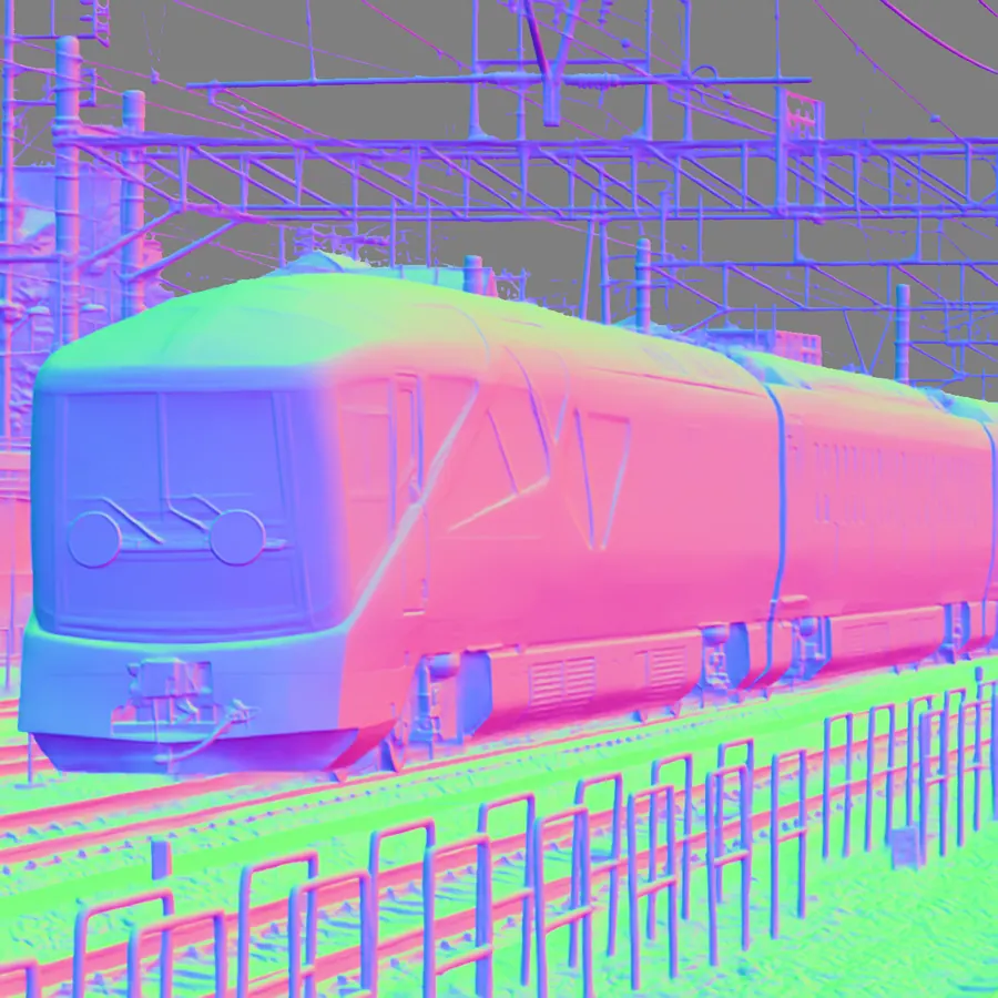
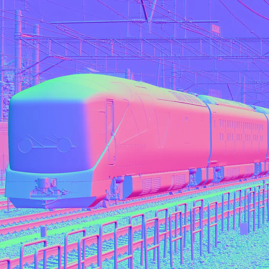
Table 9's numbers are more mixed than the depth table: Marigold V2 wins NYUv2's accuracy (61.2 vs. FE2E's 59.6) and ties Sintel's mean error with Lotus-2 (28.7 vs. 27.6, actually a hair worse), but FE2E has the better mean angular error on three of four normals benchmarks. The paper does not claim a normals sweep the way it does for depth, and the numbers support that restraint.












Albedo is the one Table 11 result that is unambiguous: Marigold V2 posts the best PSNR (20.78 vs. IID-in-the-wild's 19.28) and best LPIPS (0.195 vs. RGB↔X's 0.200) on HyperSim's intrinsic-decomposition test split, while landing second on SSIM behind IID-in-the-wild (0.811 vs. 0.819) — a genuine, not-cherry-picked win on two of three metrics.
Website, demo, repo: three different links
The link in the paper's abstract —
huggingface.co/spaces/huawei-bayerlab/marigold-v2-web —
is a static Space: a project page (sdk: static), not something you can
run inference on. The actual runnable demo lives at a different Space,
toshas/Marigold-V2. It
is easy to conflate the two since both are officially linked from the
paper's own shields, but only one of them takes an image.
The repository's own README checklist is candid about what is not out yet:
- [ ] Depth completion code
- [ ] See-through evaluation
- [ ] Diffusers integration
- [ ] ComfyUI plugin
That first line matters for how much of Section 5.1's depth-completion result (Table 7 — the test-time LoRA fit to sparse measurements, 21.2M trainable adapter params) is currently reproducible: the paper reports the numbers, but the code that produced them is not in this release. The same is true of the see-through evaluation harness — Table 8's numbers above come from the paper, not from a script in the repo I could point you at and run.
What I make of it
- The two real contributions hold up. iREPA-depth's target-not-input framing is a genuine, small, well-motivated idea, and SinkLoss's block-local optimal-transport relaxation is a clean answer to a real problem (noisy ground truth at boundaries) rather than a rebranded perceptual loss. Both survive backbone transfer (Table 5, Stable Diffusion 1.5 and FLUX.2 klein) and both check out in the released loss code exactly as described in the paper.
- The byte-level bookkeeping is trustworthy. Every claim I could check against the actual files — the LoRA rank and parameter count, the VAE-decoder split across all nine checkpoints, the shapes inside the text embeddings — matched the paper and the model card exactly, down to individual bytes. That is a genuinely well-documented release.
- The framing outruns the arithmetic in two places. "16–26% improvement" is the best two of five benchmark columns, not a representative range — the five-way average is 12.1%. And "cost-effective"/"cheap to run" is true only against other diffusion-based depth estimators; against the field's actual efficiency frontier (a plain ViT under 350M parameters), this is a 20B-parameter model that needs 17–29 GB of VRAM.
- There is real, harmless waste in the release. ~815 MB of one text-embedding file and a 3.5 MB iREPA head per checkpoint are shipped but never read by any code path in this repo, because every config hardcodes batch size 1. None of it breaks anything; all of it is checkable, which is the point.
Sources: Marigold V2 (arXiv 2609.08084) · GitHub — huawei-bayerlab/marigold-v2 · Weights — huawei-bayerlab/marigold-v2-0 · Project website · Runnable demo · Marigold V1 (arXiv 2312.02145) · REPA (arXiv 2410.06940) · Depth Anything V2 (arXiv 2406.09414) · LayeredDepth-Syn (arXiv 2503.11633).