2026-10-06 · 31 min · infrastructure · optimization · gpu
Why read this
Hightop 30%Rebalancer from source: each graph node prices its own move and writes its own MIP, SQUARES is x^1.1, plus a local-search toy and a when-to-use table.
- Runs on a laptop CPU
- A guide you can follow today
- Original analysis
Developer tools & infraApache-2.0Practitioner tool
How this was scored
- Is it new?
- 1 of 3: An incremental tweak
- Can I trust it?
- 2 of 3: Measures key facts from files, code or configs
- Can I run it?
- 3 of 3: Open, permissive, runs on reader hardware with instructions
- Will I understand it?
- 2 of 3: Mechanism from first principles with figures
- Can I act on it?
- 3 of 3: A decision guide a practitioner can follow today
- Will it last?
- 2 of 3: A reference for a year or more
- Does it affect many?
- 1 of 3: A specialist community
- Only here?
- 2 of 3: A teardown or measurement few others did
Score 69 of 100, ranked 103 of 445 rated articles. Each question is answered 0–3 by hand, and a 3 is rare. How articles are scored
Every placement system I have worked on started as twenty lines of greedy code. Put the job on the least-loaded GPU node. Then someone needs replicas spread across racks, so there is a second pass. Then a rule about not moving more than a few jobs per minute, then a rule about keeping a tenant's jobs on one NVLink island, and a year later nobody can say which rule wins when two of them disagree.
Meta's paper on Rebalancer tells the same story about its own sharding system. Shard Manager ran on hand-written heuristics for years, got a clean heuristic rewrite, and still could not balance load, because "iterative tuning of the heuristics required constant code changes that might not lead to positive outcomes and often became dead code later." The rewrite was abandoned and the team moved to Rebalancer.
On 21 September Meta open-sourced Rebalancer under Apache 2.0. The announcement on X carries three numbers: about 40 million assignment problems solved a day, more than 30 problem formulations, and a P99 solve time of 12 seconds on a problem with 265k objects and 3.2k bins. I wanted to know what the solver actually does. So I shallow-cloned facebook/rebalancer and read the C++ core, the specs and the docs, and read the OSDI'24 paper next to it.
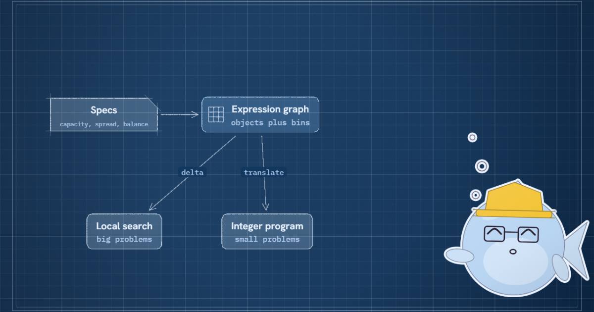
I expected a nice declarative front end on top of Gurobi, with a heuristic bolted on for when Gurobi gives up. The marketing diagram has that shape. The code is more interesting. The front end compiles to a graph, and every node of that graph knows two things about itself: how its value changes when one object moves, and how to write itself down as linear constraints. The two solvers are just two readers of the same graph.
- license
- Apache-2.0
- branch
- main
- tests
- 435 files
- source
- 10.0 MB
- commit date
- 2026-10-06
by size of tracked source at this commit, file counts in brackets; docs, data and vendored trees excluded
Read at 1a8d7f8 (6 October 2026), version 1.0.4. C++ core under algopt/rebalancer; Python wheels on PyPI as rebalancer.
local clone, 2026-10-06 at 8e25545 — branch, commit, commitDate, fileCount, hasTests, languages, license, licenseFile, shallow, testFileCount
shallow clone: counts describe the pinned tree, not the history
The problem, and why MIP alone runs out of room
An assignment problem has objects and bins. Every object goes in exactly one bin. You want to minimise some objectives without breaking some constraints. Meta's examples are racks into datacenter positions, servers into service reservations, tasks onto servers, shards onto processes, and user traffic onto regions.
The textbook way to solve it is a mixed-integer program. Introduce a binary that is 1 when object is in bin . The CPU used on bin is then a weighted sum over all objects:
Equation 1 of the paper, and the start of the trouble. Each bin's utilisation mentions every object, so the model has variables before you write a single constraint. The paper's service-placement instances are around 700k servers by 5.7k reservations. That product is about four billion binaries. The largest sharding problem is 1.8M shards on 27k servers, which is about 49 billion. No solver is getting through that inside the five-minute deadline that sharding has.
The paper's answer is to stop writing the problem as a MIP in the first place, and only produce one when it is small enough to be worth it.
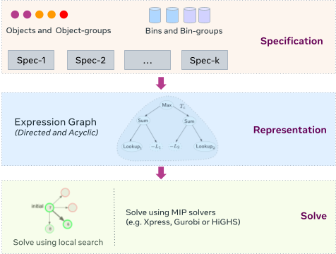
Specs are recipes over four nouns
Rebalancer's modelling language has four nouns. A dimension maps every object and every bin to a number: CPU per task, CPU capacity per server. A scope groups bins: servers into racks, racks into power domains. A partition groups objects: tasks into jobs, shard replicas into replica sets. Utilisation is equation 1, lifted to any scope item and any object group.
On top of those sit the specs, which are canned objectives and constraints. The blog's example is the paper's Figure 1, redrawn:
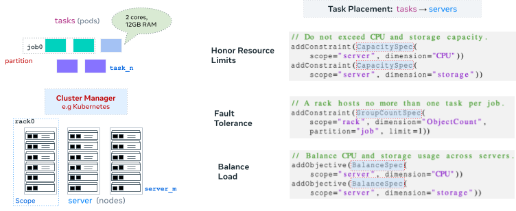
The open-source Python API looks like this. It is the README's own quick example: four tasks of 10 memory each, two hosts of 20, and host0 starting with three of them.
# README.md, "Quick Example" (facebook/rebalancer @ 1a8d7f8)
from rebalancer import ProblemSolver
from rebalancer.specs import (
    CapacitySpec, ConstraintSpec, LocalSearchSolverSpec,
    MoveTypeSpec, SingleMoveTypeSpec, SwapMoveTypeSpec, SolverSpec,
)

solver = ProblemSolver(service_name="rebalancer", service_scope="example")
(solver
    .set_object_name("task")
    .set_container_name("host")
    .set_assignment({"host0": ["task0", "task1", "task2"], "host1": ["task3"]})
    .add_object_dimension("memory", {"task0": 10, "task1": 10, "task2": 10, "task3": 10})
    .add_container_dimension("memory", {}, default_value=20.0)
    .add_constraint(ConstraintSpec(capacitySpec=CapacitySpec(
        name="memory_capacity", scope="host", dimension="memory")))
    .add_solver(SolverSpec(localSearchSolverSpec=LocalSearchSolverSpec(
        moveTypeList=[MoveTypeSpec(singleMoveTypeSpec=SingleMoveTypeSpec()),
                      MoveTypeSpec(swapMoveTypeSpec=SwapMoveTypeSpec())])))
)
solution = solver.solve()
You never write . You never write a big-M. You name a scope and a dimension and the spec builder emits the formula.
The spec catalogue has grown since the paper. The OSDI'24 version lists 21 frequently used specs out of 28. At this commit the Thrift ConstraintSpecs union has 36 members and GoalSpecs has 37, and there are 48 spec builders in materializer/spec_builder/. The paper also reports that 85% of constraints and objectives across its use cases reuse an existing spec without touching the lower-level expression API, and an average problem uses seven specs, with a maximum of 14. The usability claim rests on that 85%, and it is the one number I can't check from outside Meta.
Utilisation has a time axis
One modelling idea is worth stopping on, because it is what makes Rebalancer usable for migrations and not only for green-field placement. Utilisation is defined over three sets of objects: the ones in a bin now (AFTER), the ones in it at the start (INITIAL), and the ones that never left (STAYED). Subtracting gives the useful variants. NEW is AFTER minus STAYED, the objects that arrived. OLD is INITIAL minus STAYED, the ones that left. ANY is INITIAL plus AFTER minus STAYED, everything that was in the bin at any point.
ANY is double occupancy. When Shard Manager moves a shard, it loads it on the destination before dropping it from the source, so for a while it costs memory on both. A CapacitySpec over ANY says "this server must fit its shards even mid-migration." NEW and OLD with an object-count dimension give you churn limits. In the code ANY is called DURING ("final + initial - stayed" in the utilisation docs), next to AFTER, NEW, OLD and MOVED, and CapacitySpecBuilder.cpp maps a DURING_AND_AFTER capacity definition onto two checks. If you have ever written "and also don't OOM the target node while copying weights to it" as a special case in a scheduler, this is that special case, made a parameter.
Two things in the specs I did not expect
BalanceSpec defaults to the LINEAR formula. Reading BalanceSpecBuilder.cpp, that is the mean positive deviation above the average relative utilisation:
The option named SQUARES is not a square. Lines 164 to 180 of BalanceSpecBuilder.cpp apply power(expr, 1.1) to each utilisation and the threshold. An exponent of 1.1 penalises the hottest hosts slightly more than linear without the steep curve of a real square. I suspect it was tuned on production problems and the enum name never followed. If you pick SQUARES expecting variance-like behaviour, you get something much closer to LINEAR. There is a separate RELATIVE_UTIL_VARIANCE formula for that.
The second surprise is how broken constraints are handled. A real cluster is rarely feasible when you start: a host is already over its limit, a rack already holds two replicas. A hard constraint would make the whole problem infeasible. Rebalancer's DEFAULT constraint policy, documented in website/docs/reference/constraint-policy.md, splits an initially broken constraint into two pieces. "Do not make it worse than it started" stays hard. "Fix it" becomes a goal in tuple position 0:
penalty = invalidCost  * (amount by which the constraint is violated)    # default 100
        + invalidState * step(violation)                                  # default 10000
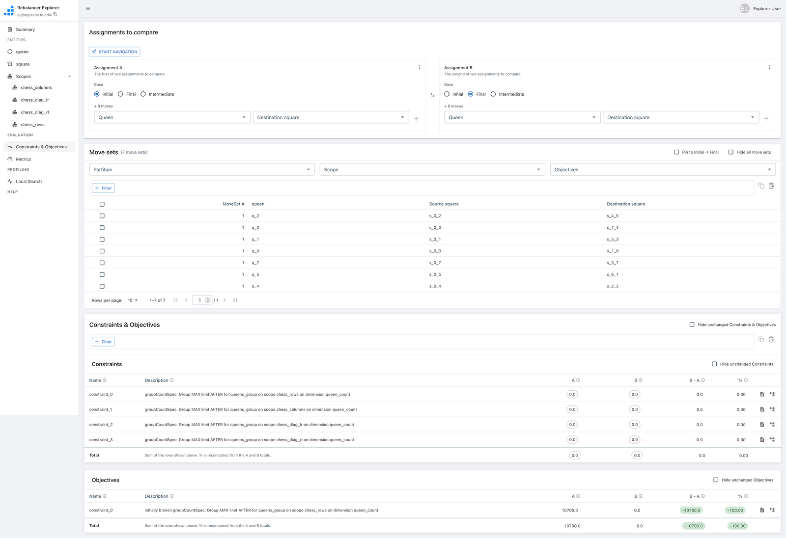
The 100 rewards each unit of progress. The 10000 is a cliff that rewards finishing the job. The Explorer screenshot in the repository shows it on the eight-queens example: an "initially broken groupCountSpec" on chess rows at 10700. With all eight queens in one row and a limit of one per row, the violation is seven, and 10000 plus 100 times 7 is 10700. The number on the screen is the formula.
The graph
Once the specs are in, Materializer turns them into an expression graph. Leaves are utilisations. Interior nodes are Sum, Max, Step, Power, Piecewise, SumOverThreshold and about 40 other expression types under solver/expressions/. A constraint is an inequality , and a whole CapacitySpec over servers collapses into one node, .
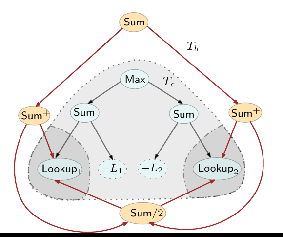
The node that makes the size instead of is ObjectLookup. Its observation is that a task needs the same memory whichever server it lands on. So there is one shared vector per dimension, object to value, and a lookup node holds only a pointer to that vector and to its set of bins. The comment at the top of ObjectLookup.cpp says it plainly: "From mathematical perspective, ObjectLookup is a linearsum. The difference is: It is implemented in an efficient way to save memory and complexity among those who share the same linearsum equation."
The lookup prices a candidate move like this. A ChangeSet is a list of (object, bin, +1 or −1) entries. A single move is two of them.
// algopt/rebalancer/solver/expressions/ObjectLookup.cpp:401-424
double ObjectLookup::evaluate(
    const BottomToTopEvaluator& /* evaluator */,
    const ChangeSet& changes) const {
  double delta = 0;
  const auto& objVec = *object_vector;
  if (changes.size() <= containersPtr_->size()) {
    for (const auto& change : changes) {
      if (containersPtr_->contains(change.getContainer())) {
        delta += change.getValue() * objVec.getObjectValue(change.getObject());
      }
    }
  } else {
    for (const auto containerId : *containersPtr_) {
      for (const auto& change : changes.getChangesByContainer(containerId)) {
        delta += change.getValue() * objVec.getObjectValue(change.getObject());
      }
    }
  }
  // ...
  return value + delta;
}
It never re-sums the bin. It adds the moved object's value to the cached total. Two hash lookups and a multiply.
The interior nodes do the same trick for their own operator. Max keeps its children in a sorted container. On evaluation it takes the max over the children that changed, then walks the sorted list only until it finds the largest child that did not change:
// algopt/rebalancer/solver/expressions/Max.cpp:110-141 (trimmed)
double Max::evaluate(const BottomToTopEvaluator& evaluator,
                     const ChangeSet& changes) const {
  double new_max = -1 * numeric_limits<double>::max();
  auto& changedChildren = evaluator.getChangedChildren((Expression*)this);
  for (auto child : changedChildren) {
    const double val = evaluator.evaluate(child, changes);
    if (val > new_max) new_max = val;
  }
  if (changedChildren.size() == children().size()) return new_max;
  // largest child that hasn't changed: first unchanged entry in sorted order
  for (const auto& [child, val] : sorted_values_) {
    if (!changedChildren.contains(child)) {
      if (val > new_max) new_max = val;
      break;
    }
  }
  return new_max;
}
The paper's "minimal computation during a node update" fits in about 30 lines. A capacity constraint over 3.2k servers, asked about a move between two of them, looks at two children and usually one more entry of a sorted list. SumOverThreshold, which backs the balance formula, keeps its children in an aggregate structure of sums, sums of squares and counts, so when the average itself moves it can recompute the sum above the new threshold without a full pass.
What decides which nodes get asked is the Orchestrator. At init it walks the graph post-order, gives every node a priority (its root, then its height), records parents, and builds maps from bins and objects to the leaves they touch. To price a move it pushes the touched leaves into a priority queue and pops them bottom-up. A node whose value changes notifies its parents, and a parent enters the queue the first time one of its children reports a change:
// algopt/rebalancer/solver/expressions/Orchestrator.cpp:360-377 (trimmed)
void Orchestrator::notifyChange(Context& context, Expression* changedNode) const {
  auto parentsPtr = folly::get_ptr(nodeToParents_, changedNode);
  if (parentsPtr) {
    for (auto& parent : *parentsPtr) {
      auto& changedChildren = context.changedChildren()[parent];
      if (changedChildren.empty()) {
        context.readyNodes().emplace(priority(parent), parent);
      }
      changedChildren.insert(changedNode);
    }
  }
}
The evaluate call above it (lines 269 to 305) stops as soon as it has the value of the node that was asked for. That matters because of the order in which MovesEvaluator::evaluate asks:
// algopt/rebalancer/solver/moves/MovesEvaluator.cpp:203-229 (trimmed)
MoveResult MovesEvaluator::evaluate(MoveSet&& moves) const {
  static thread_local Context context;
  context.clear();
  context.changes() = moves.getChangeSet();
  // Step 1: check constraint. If positive, the move is invalid.
  if (isPositive(problem_.getLabeledConstraints(), context)) { return MoveResult::makeInvalid(...); }
  // Step 2: check "do not make worse" goal. If worse, the move is invalid.
  if (auto worseTuplePos = doNotWorsenGoalConfig_.getFirstWorseTuplePos(context, ...)) { ... }
  // Step 3: evaluate minimizing goal.
  auto newValue = minimizingGoal_.evaluate(context, problem_.getOrchestrator());
  ...
}
Constraints are checked first, then higher-priority goals that must not get worse, and only then the objective being minimised. A move that overloads a host is rejected after pricing the capacity subgraph and nothing else. Most candidate moves are bad moves, so most evaluations end at step 1. The thread_local context is the other detail to notice: evaluation never mutates the graph, so it parallelises without locks.
The objective itself is a tuple compared lexicographically, set up with add_goal(spec, weight, tuple_pos) and add_goal_boundary(). Within a tuple slot, goals are a weighted sum. That gives you strict priorities ("fix capacity before you care about balance") without inventing weights of 1e6 and hoping.
Local search, the part that runs at Meta's scale
The blog is direct about which solver matters: "At Meta, almost all large-scale problems use local search." The loop is in CoreLocalSearchSolve.cpp, and it is short:
// algopt/rebalancer/solver/solvers/CoreLocalSearchSolve.cpp:546-574 (trimmed)
do {
  solveState_.startNewCycle();
  while (auto hotContainer = solveState_.hotContainerSelector_.next(
             solveState_.skipContainers)) {
    if (!improveHotContainer(*hotContainer, lastImprovedTime)) {
      solveState_.skipContainers.insert(*hotContainer);
    } else {
      solveState_.unfixableContainers.clear();
    }
    if (reachedGlobalOptimum()) return finalizeAndReturn(true);
    else if (shouldTerminate(timer_.getSeconds(), lastImprovedTime)) return finalizeAndReturn(false);
    else if (reachedLocalOptimum()) break;
  }
} while (shouldStartNextCycle());
Three ideas carry it.
The first is that search is organised by bin, not by object. The paper's reasoning is that bins are usually far fewer than objects, so "restricting the search by bins makes faster local progress." Take the hottest bin, try moving things out of it, apply the best move, re-rank.
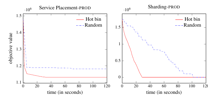
The second is how "hottest" is defined. Each node keeps a potential, its current value minus its lower bound. A potential of zero means that subgraph is already optimal. PreOrderExpressionIterator walks down from the objective root, pushing children in order of potential and dropping any child whose potential is zero (ExpressionIterator.cpp:93-105). The bins attached to the leaves it reaches first are the hot ones. The graph is the index of where the objective is losing. The paper's Figure 6 shows what that buys on two production problems: the same local search with random bin order takes about 100 seconds to get the sharding objective to zero, and hot-bin order gets there in about 30.
The third idea is that a "move" is pluggable. For each hot bin, improveHotContainer tries the configured move types in list order and applies the best move of the first type that strictly improves the tuple (lines 394 to 442). SINGLE tries every object in the hot bin against every other bin. SWAP exchanges an object with one in another bin. KL_SEARCH builds a Kernighan–Lin style chain. The paper's SINGLE_RANDOM samples destinations, and it found a 10% sample capped at 1k bins a good trade on 100k-node clusters. There are 29 move types under solver/moves/ at this commit, and the docs recommend starting with single, swap and triple loop.
Parallelism lives inside a move type. AsyncSingleMovesMoveType dedupes the hot bin's objects by equivalence set, filters destinations to accepting bins, and hands the cross product to a thread pool:
// algopt/rebalancer/solver/moves/AsyncSingleMovesMoveType.cpp:37-76 (trimmed)
const auto dedupedObjs =
    ObjectDeduper(&problem.getEquivalenceSets(), dynamicObjects);
...
return folly::coro::blockingWait(
    CoroUtils::parallelMapReduceAllPairs(
        filteredObjects, filteredContainers,
        [&](entities::ObjectId hotObject, entities::ContainerId coldContainer) {
          return exploreFromAllSingleMoves(
              evaluator, hotContainer, hotObject, coldContainer, stats);
        },
        [](MoveResult& bestResult, MoveResult&& batchResult) {
          bestResult.aggregate(std::move(batchResult));
        },
        []() { return MoveResult::makeEmpty(); },
        evaluator.getProblem().configs.threadPool));
The dedupe is the equivalence-set idea from the paper. If three tasks of the same job sit on one server and every spec treats them identically, moving any of them is the same move, so only one is tried. Equivalence sets are computed from the graph itself: Orchestrator::updateEquivalenceSets walks the nodes post-order and each node splits the sets it can tell apart.
The paper's numbers for the whole machine: roughly 150k evaluations a second on most large instances. On one large sharding problem, parallel evaluation reached 170k evaluations a second and 12k applied moves in a 300-second limit, against 25k evaluations a second and 2k moves sequentially. On the Kubernetes benchmark, all 50k candidate moves for one pod were evaluated in 100 ms.
A toy you can step through
I reimplemented the loop on a problem small enough to watch. Twelve tasks, four jobs of three replicas, six hosts of 10 CPU in three racks. Job A tasks take 4 CPU, B take 3, C take 2, D take 1, so there are 30 CPU of work and the mean host sits at 5. Someone has piled jobs A and B onto rack 0: host 0 holds 14 CPU and rack 0 holds all three replicas of both jobs.
Both the capacity and the one-per-rack constraints start broken. Under the DEFAULT policy each becomes a fix-it goal in tuple position 0. Capacity is over by 4 and the spread rule by 7 (two surplus replicas each of A and B in rack 0, plus one of C and two of D in rack 1), so the starting goal is 100 times 4 plus 10000, plus 100 times 7 plus 10000, which is 21100. Balance, the LINEAR formula times 60 so it stays an integer, sits in tuple position 1.
Start: host 0 holds 14 CPU against a limit of 10, and rack 0 holds all three replicas of job A and of job B. Both constraints are broken, so each becomes a fix-it goal of 100 × violation + 10000 in tuple position 0: capacity is over by 4 and the spread rule by 7, which gives 21100.
With hot-host order and SINGLE moves only, the first move takes A0 from host 0 to host 3. That one move clears the capacity violation, takes a spread violation off, and drops the goal to 10600. The first constraint's 10000 cliff is gone. Seven moves and 75 evaluations in, both constraints hold and the fix-it goal is 0. Two moves later, after 100 evaluations in total, it stops with hosts at 4, 6, 5, 5, 5, 5. Host 1 holds a 4 and a 2, and no single move out of it, or out of any other host, strictly improves the tuple. It is stuck in a local optimum, the failure mode the local-search docs warn about in their "Cons" list.
Switch on SWAP and the solver, stuck on host 1, swaps A2 with B1 between host 1 and host 0, then finishes with all six hosts at 5 after 116 evaluations. Random host order also gets there in this case, but takes 10 moves and 235 evaluations. On a toy this small the evaluation count barely matters. The paper's Figure 6 is the same effect at a scale where it does.
The toy leaves out the parts that make the real one fast, which are the incremental graph, the parallel evaluation and sampled destinations. Its evaluate function recomputes everything from scratch. It shares the decision structure: hot first, move types in order, a lexicographic tuple, broken constraints as goals that may never get worse.
The MIP side reads the same graph
The other half of every expression class is an lp() method. It is the paper's mipTranslate, and it emits the node as linear constraints over assignment variables. Here is the lookup:
// algopt/rebalancer/solver/expressions/ObjectLookup.cpp:347-361 (trimmed)
auto expr = evaluator.makeLpExpression();
double rawSum = 0;
for (const auto& [equiv_set, coef] : evaluator.getEquivSetMap(object_vector)) {
  for (auto container : *containersPtr_) {
    if (auto fixedValue = evaluator.getMaybeFixedAssignmentValue(equiv_set, container)) {
      rawSum += coef * fixedValue.value();
    } else {
      expr += coef * evaluator.getAssignmentVar(equiv_set, container);
    }
  }
}
expr += rawSum;
return expr;
Look at what the variable is indexed by. It is an equivalence set and a container, not an object and a container. LPStore::reset creates them as integer variables named assign_<set>_<container> (LPStore.cpp:119-134). The blog calls this "variable aggregation, compacting similar objects into a single integer variable." If 1,000 identical tasks can go on 50 hosts, you get 50 integers that count tasks per host rather than 50,000 binaries. The same equivalence sets that dedupe local-search moves shrink the MIP, which is a nice bit of reuse.
Max::lp shows the cost of nonlinearity. When the max is being minimised, one continuous variable bounded below by every child is enough. When it is being maximised, you need a binary per child and a big-M, and the code refuses to build a model with a silly one: if (bigM >= LARGEST_VALUE) throw std::runtime_error("Huge bigM calculated, model won't be correct.");, with LARGEST_VALUE set to 1e8 (Max.cpp:405-408). Some specs cannot be translated at all. A BalanceSpec with the CAPACITY_PER_ITEM metric throws "not currently supported with the OptimalSolver ... use LocalSearch instead," because it divides by an object count. The two readers of the graph do not have the same reach, and the code says so loudly rather than quietly producing a wrong model.
Bars are drawn on a digit scale. Aggregating identical objects into one integer variable per bin shrinks the MIP by exactly the dedup ratio, but it is still a product with the bin count; the graph grows with the sum. The dedup share is a dial: nobody has published what a production problem collapses to.
Even with aggregation, the MIP is a product of sets and bins. The graph grows with the sum. That asymmetry is the whole argument for local search at Meta's scale, and the paper measures the graph side: on three sharding instances of 71k, 152k and 289k objects, graph memory grew from 1.7 GB to 3.2 GB to 6.2 GB. Linear, as claimed, and also about 21 KB per object, which is not tiny. Budget memory accordingly if you feed it a million objects.
There are two more solvers in solver/solvers/ that the blog does not mention. OptimalSubsetSolver repeatedly picks a subset of containers, freezes everything else, and solves that piece as a MIP with a default of 0.5 seconds per subset. In other words, large neighbourhood search with an exact inner solver. ChainSolver runs whatever solvers you add in sequence on the same problem, so "local search for 60 seconds, then polish with subset MIP" is two add_solver calls. The paper describes a POP-like partitioned MIP that Meta used in production for service placement before switching. I would guess the subset solver is its descendant, but that is my reading of the code, not something either source says.
Two practical notes on the open-source build. OptimalSolverSpec.solverPackage defaults to XPRESS. The CMake build has Xpress and Gurobi off by default and defines REBALANCER_SOLVER_FALLBACK_TO_HIGHS_ONLY at CMakeLists.txt:197, so an unconfigured optimal solve logs "Failed to load solver XPRESS" and falls back to HiGHS. It works, but set solverPackage to HIGHS yourself and skip the error in your logs.
What the evidence says
The production numbers moved between the paper and the blog, in the right direction. The 2024 paper, sampling a typical week of production solves, gives P99 solve time as 16 s on 65k objects and 5k bins. The blog (2026) gives P99 12 s on 265k objects and 3.2k bins, and for problems above 1M objects and 5k bins an average of 171 s over more than 3.4k runs. 40 million problems a day is about 460 every second. The blog does not say how many cores a solve gets, so I can't turn the 12 s into anything per core.
On quality, the most useful table is Table 3: local search against Meta's own partitioned MIP on four production service-placement instances. Local search takes 146 to 214 seconds against 350 to 557 for the partitioned MIP, and its objective is worse by 0.11% to 0.56%. The paper's "up to four times faster" is the 645k by 4.5k row, 146 s against 557 s.
Table 2 is the stress test. On 10k Azure pods and 500 nodes, the optimal MIP places 94.6% of pods in 31 ms per pod, SINGLE_GREEDY places 92.8% in 8 ms and SINGLE_RANDOM 93.2% in 6 ms. The authors also built a pathological case where the only full placement packs every node to exactly 32 GB. At N = 10 the MIP places 100% of pods in 209 ms and local search 97.1% to 97.8% in under a millisecond. At N = 100 the MIP timed out after 600 s, and local search still placed 97.4% to 97.7%. So the trade looks like this: you give up a couple of percent on adversarial packing to get an answer at all.
Against OR-Tools and a plain MIP
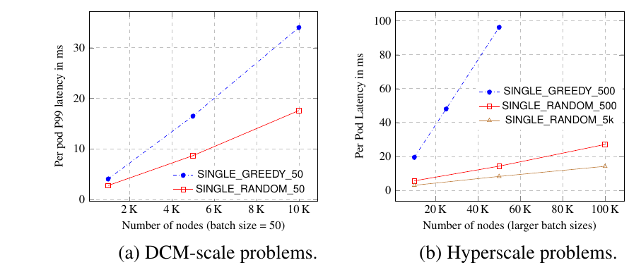
The obvious reply on X was "what's the benefit over directly using open-source LP/MIP solver libraries?" The paper's closest comparison is DCM, which compiles SQL-like scheduling policies into a constraint problem for OR-Tools' CP-SAT. DCM's paper tops out at 50 pods per batch on 10k nodes at close to 30 ms per pod. Rebalancer's SINGLE_RANDOM reaches 14 ms per pod on 100k nodes with batches of 5k. Two caveats come from the paper itself. The DCM numbers are quoted from the DCM paper, not rerun, because neither system could run on the other's machines. And Rebalancer's Kubernetes policies took about 500 lines against DCM's 550 lines of SQL, so the expressiveness claim is "comparable," not "better."
Here is how I'd place the options for an ML-infra team:
| Model size | Optimality | Good at | Bad at | |
|---|---|---|---|---|
| Hand-written greedy | none | none | sub-millisecond decisions | adding the fifth policy |
| MIP via HiGHS, Gurobi, PuLP | objects × bins | proven, given time | hundreds to tens of thousands of objects, deadlines in minutes | millions of objects, nonlinear goals, stable re-solves |
| OR-Tools CP-SAT | objects × bins, plus propagation | proven, given time | combinatorial side rules, small and medium instances | the same scale wall as MIP |
| Rebalancer, MIP backend | equivalence sets × bins | proven, given time | the above, without writing the model | the same scale wall, less of it |
| Rebalancer, local search | objects + bins | none, local optimum | 100k to 1M+ objects, incremental rebalancing, churn limits | moves that only work when several objects shift together |
The reason to pick Rebalancer over raw HiGHS is not raw speed on one solve. It is that the model is written once, at the level of "capacity on hosts, spread across racks," and you can move between backends as the problem grows. Meta's service placement did exactly that, from MIP to partitioned MIP to local search, and the paper is unusually frank about it: "despite having the local search technology, our unwavering faith in MIP's optimality led us on a lengthy detour to reach our current state." A system I can rewrite from one backend to another by changing one add_solver call is worth a lot more than 0.5% of objective.
Local search is also more stable across re-solves, which matters for anything that runs every few minutes. It only applies strictly improving moves, so an already-good assignment stays put. A MIP solver that finds two solutions of equal value may return either, and the paper says they add MinimizeMovementSpec for exactly that reason when using MIP.
Where I'd put it in an ML stack
GPU job placement is the first fit. Training jobs are objects with GPU-count, GPU-memory and host-memory dimensions. Nodes are bins, scoped into NVLink domains, racks and power domains. Capacity is CapacitySpec. Keeping a job's ranks inside one rack or one switch domain is ColocateGroupsSpec over a job partition. Spreading inference replicas across failure domains is GroupCountSpec. Not disturbing running jobs is MinimizeMovementSpec, or AvoidMovingSpec for jobs that must not move at all. A defragmentation pass, freeing whole nodes for an 8-GPU job, is ToFreeSpec on the nodes you want empty. A sketch of that model in the Python API follows. I have not run it, since I did not execute the package, so read the field names as taken from src/rebalancer/specs.py and the call shapes from _rebalancer.pyi:
# sketch, not run: field names from src/rebalancer/specs.py at 1a8d7f8
solver = ProblemSolver(service_name="gpu-pool", service_scope="rebalance")
solver.set_object_name("job").set_container_name("node")
solver.set_assignment(current)                       # node -> [jobs]
solver.add_object_dimension("gpus", job_gpus)
solver.add_container_dimension("gpus", node_gpus)
solver.add_scope("nvswitch", node_to_switch)
solver.add_scope("rack", node_to_rack)
solver.add_partition("tenant", tenant_to_jobs)

solver.add_constraint({"capacitySpec": {"name": "gpu_cap", "scope": "node", "dimension": "gpus"}})
solver.add_constraint({"groupCountSpec": {"name": "spread", "scope": "rack",
                                          "partitionName": "tenant",
                                          "limit": {"type": "ABSOLUTE", "globalLimit": 4}}})
solver.add_goal({"balanceSpec": {"name": "bal", "scope": "nvswitch", "dimension": "gpus"}})
solver.add_goal_boundary()                           # strictly lower priority below
solver.add_goal({"minimizeMovementSpec": {"name": "churn", "scope": "node", "dimension": "gpus"}})
Shard placement is the second fit, and the one Meta built it for. Embedding-table shards for a recommender, KV-cache or model-weight shards for a serving tier, vector-index shards: objects with memory and QPS dimensions, processes or hosts as bins, ANY utilisation so a migration never overcommits the target, and per-server churn limits through NEW and OLD counts. The paper's sharding instances, 1.8M objects on 27k bins under a five-minute deadline, are bigger than anything I run, and in production 90% of those solves finish within 10 seconds.
Inference serving placement is the third. The paper lists "minimizing the number of replicas for ML inference models or databases deployed across geo-distributed datacenters, while adhering to latency SLO and meeting varying user request rates" among its use cases, and the message-queue example shows the pattern: AssignmentAffinitiesSpec with negative latency as affinity, DrainCapacitySpec to keep enough headroom for any one region failing. Map models to regions, or LoRA adapters to replicas, and you have the same problem. The site's write-ups on vLLM, SGLang and Prime Inference are all about what happens inside one serving replica. This is the layer above, deciding which replica serves what.
The same shape turns up in DSec's placement engine, which packs 50× overcommitted agent sandboxes onto nodes, and in FreeVideo's planner, which places a video transformer's blocks across memory tiers.
Where I would not use it is anything per request or per batch. Balancing tokens across mixture-of-experts GPUs every step needs microseconds, and the paper's own recommendation is that "systems requiring short and predictable latency in resource allocation decisions should use ad hoc heuristics." Rebalancer belongs in the control loop that runs every few minutes: the periodic expert re-placement, not the router.
Rough edges
It is a big C++ dependency. A source build needs fbthrift and folly built first. The Linux wheel for 1.0.4 on PyPI is 99.8 MB, oddly close to PyPI's 100 MB per-file limit, even though the 1.0.1 changelog says stripping debug symbols brought wheels to about 13 MB. Binary wheels exist only for CPython 3.12 to 3.14. Some of the internal origin shows: examples/README.md still documents buck2 run @fbcode//... targets, and examples/tupperware/tupperware.py imports from algopt.rebalancer.interface.py_client, a path the public package does not have.
The bigger limit is the one the docs state honestly. Local search finds local optima, and it is weakest when progress needs several objects to move together, the "container A must contain either 5 or 8 objects exactly" case in the local-search docs. My toy hit a mild version of it with SINGLE alone. The fixes are a richer move type or a subset-MIP pass on top, and both exist, but you have to know to reach for them. Rebalancer Explorer exists for that. The blog says modellers' time "shifted to debugging the solver's behavior," and the Explorer answers the useful questions: which constraint is binding, and why didn't this object move there.
What I take from it
The most reusable idea is not local search, which is old, or MIP, which is older. It is making each operator in the model responsible for its own incremental update and its own linearisation, and having two solvers that only ever talk to operators. A new spec is a new composition of existing operators, and a new operator gets both solvers for free once it implements both methods. It explains how one team could serve 30+ formulations for nine years.
If you run placement for a GPU cluster or a sharded serving tier and your scheduler is a growing pile of rules, I think this is worth an afternoon of modelling. Start with the MIP backend on a small slice to learn what a good answer looks like, then switch the same spec to local search. Meta's blog describes exactly that workflow.
How I checked
I shallow-cloned facebook/rebalancer at commit 1a8d7f8 (6 October 2026, version.txt 1.0.4) and read the solver core rather than the README alone: CoreLocalSearchSolve.cpp, HotContainerSelector.cpp, ExpressionIterator.cpp, Orchestrator.cpp, MovesEvaluator.cpp, AsyncSingleMovesMoveType.cpp, ObjectLookup.cpp, Max.cpp, SumOverThreshold.cpp, LPStore.cpp, OptimalSubsetSolver.cpp, ChainSolver.cpp, Materializer.cpp, the Capacity and Balance spec builders, lp/factory/ProblemFactory.cpp, the Thrift IDL and the docs under website/docs/. File and line references above are to that commit. I counted the spec builders, move types, expression files and the members of the ConstraintSpecs and GoalSpecs unions directly.
Paper numbers are from the OSDI'24 PDF (Kumar et al., pages 507 to 524); blog numbers are from the engineering post of 21 September 2026. The figures are taken from those two sources and from the repository, flattened onto white. The PyPI wheel sizes come from the package's JSON metadata.
I did not run Rebalancer: the house rule is not to execute third-party code, so every claim about behaviour comes from reading the source. The interactive toy is my own reimplementation in components/articles/meta-rebalancer/toy-solver.ts, and its move-by-move numbers (21100 at the start, 75 evaluations to a feasible assignment, the local optimum at 4, 6, 5, 5, 5, 5) are from running that file. The arithmetic I did myself is the 4-billion and 49-billion variable counts, the 460 problems a second, and the roughly 21 KB per object of graph memory. I could not check the 85% spec-reuse figure, the 40 million a day, or the 12-second P99, which are Meta's numbers from Meta's fleet.