2026-10-06 · 29 min · diffusion · diffusion-transformers · image-generation · video-generation · flow-matching · inference
Why read this
Solidtop 85%How LoT turns a layout into rectangle tokens a pretrained DiT can denoise, why images gain less than the token cut and video more, and what eval layouts leak.
- Original analysis
- A new technique
- Concrete numbers to act on
Image & video generationNothing to runResearch paper
How this was scored
- Is it new?
- 2 of 3: A real new idea, method or capability
- Can I trust it?
- 2 of 3: Measures key facts from files, code or configs
- Can I run it?
- 0 of 3: Closed, nothing to run
- Will I understand it?
- 2 of 3: Mechanism from first principles with figures
- Can I act on it?
- 2 of 3: A concrete recipe, numbers or comparison
- Will it last?
- 1 of 3: Relevant for months
- Does it affect many?
- 1 of 3: A specialist community
- Only here?
- 2 of 3: A teardown or measurement few others did
Score 55 of 100, ranked 293 of 445 rated articles. Each question is answered 0–3 by hand, and a 3 is rare. How articles are scored
Gordon Wetzstein opened his thread with a line I have been thinking about for a while: "Diffusion models spend the same compute on a blank wall as on a face. But you often know in advance where the detail will be." Brian Chao's post on the same paper adds the reason this is timely. Image models increasingly start from a plan (boxes, masks, a layout written by a language model) before a pixel exists. If the plan already says where the hard parts are, why does the transformer still give the sky the same 4,096 tokens as the eyes?
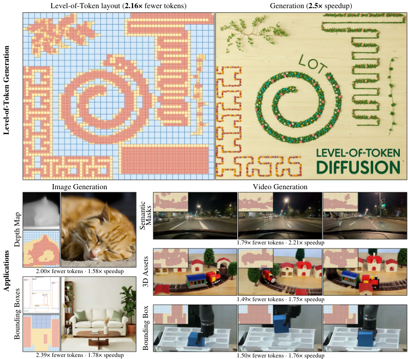
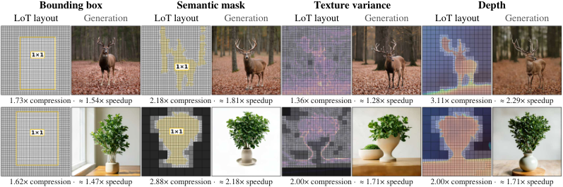
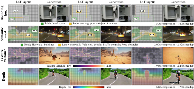
Level-of-Token Diffusion, or LoT (arXiv 2610.05816), answers that literally. It comes from Stanford, first author Kiyohiro Nakayama, with Federico Tombari of Google and Leonidas Guibas among the authors and Lior Yariv and Gordon Wetzstein as equal advisers. It tiles the token grid with rectangles of different sizes, fine where the plan says detail matters, and fine-tunes a pretrained DiT to denoise the short sequence that tiling produces. Brian's thread puts it at "2–3.5×" faster while keeping quality and control.
I expected token merging in a new coat, and was wrong. The tokens are fixed before sampling starts, so nothing is measured or merged at run time, and the whole trick rests on one piece of algebra borrowed from the same group's asymmetric flow paper, which lets an 8×8 token look at 128 numbers out of 8,192 and still return a full-resolution velocity. The second thing that surprised me came from the speed tables. On images LoT never runs as fast as its token cut suggests. On video it runs faster. That difference tells you where to use it.
There is no code and no weights. The project page is a static site whose repository (georgenakayama/lotdiffusion on GitHub) holds the demos, real token layouts as JSON and a timing file, but no model. So everything below is checked against the paper, its appendix, the project page's data files and the two base models' published configs.
A layout is a tiling of the token grid
Start from what a pretrained DiT does. FLUX.2 klein encodes a 1024×1024 image to a 128×128 latent with 32 channels, then patchifies 2×2 latent pixels into one token. Its transformer/config.json says in_channels: 128, which is those 2×2×32 numbers, and the hidden width is 24 heads of 128, so 3,072. The DiT sees a 64×64 grid, 4,096 tokens, each a 128-vector. Every one of them goes through every block at every step.
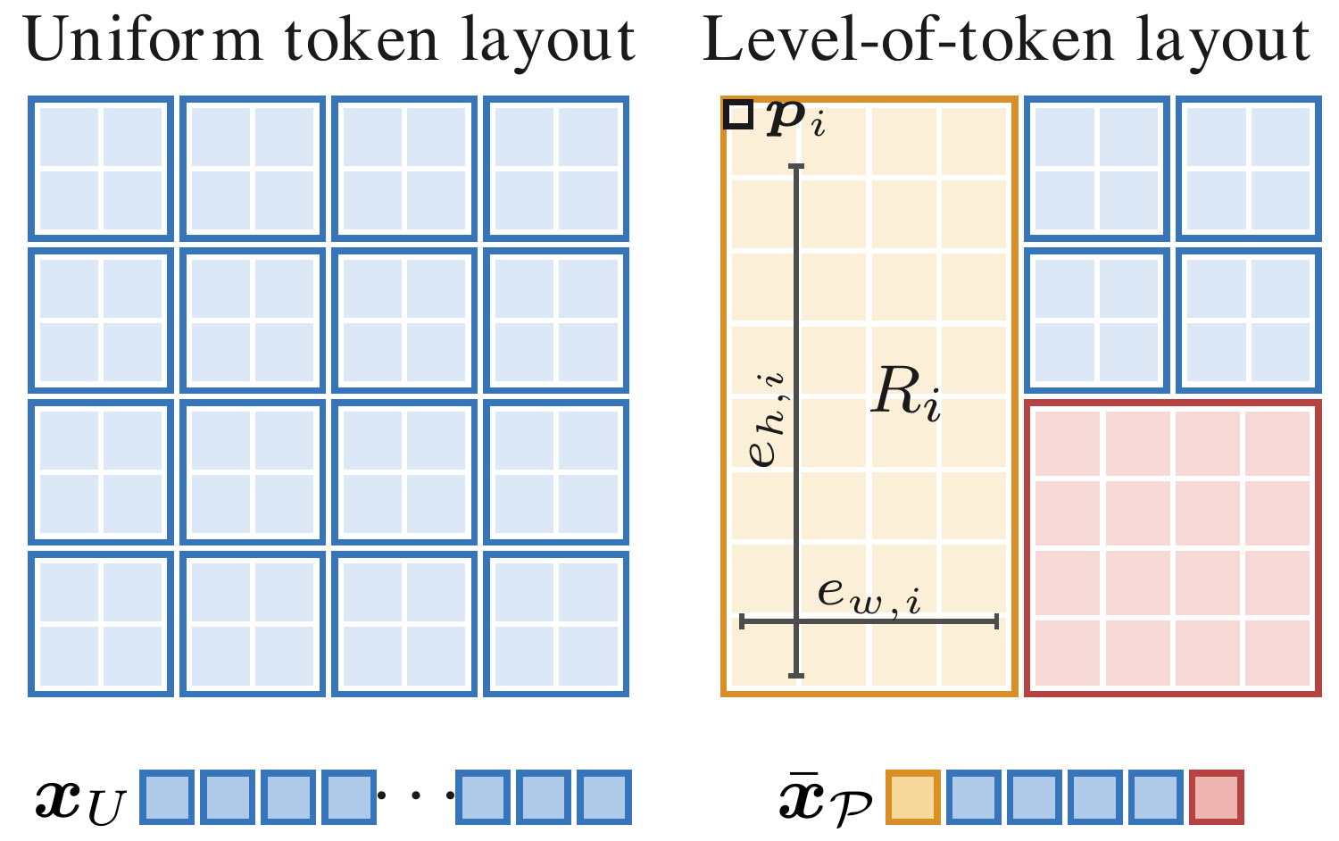
LoT keeps that grid as the finest level and lets a token cover a rectangle of it. Formally a layout is a partition of the token grid into disjoint axis-aligned rectangles
where is the top-left corner and the extent. The image model supports , which is sixteen shapes including thin ones like 1×8. The video model, built on Wan2.1, uses per spatial axis and never merges across time. The paper reports savings as token compression, for an image and for a video.
What does a real layout look like? The project page ships the exact tiling behind one of its demos, the "flowering letters" image, as a list of [x, y, w, h] rectangles on a 96×160 grid (a 1536×2560 image). I rendered it next to the generation. Five rows of the word LOT get progressively more detailed from top to bottom, from flat paint to dense jasmine, and the layout follows: 554 tokens in the top fifth, 1,122 in the bottom fifth, against 3,072 for a dense fifth.
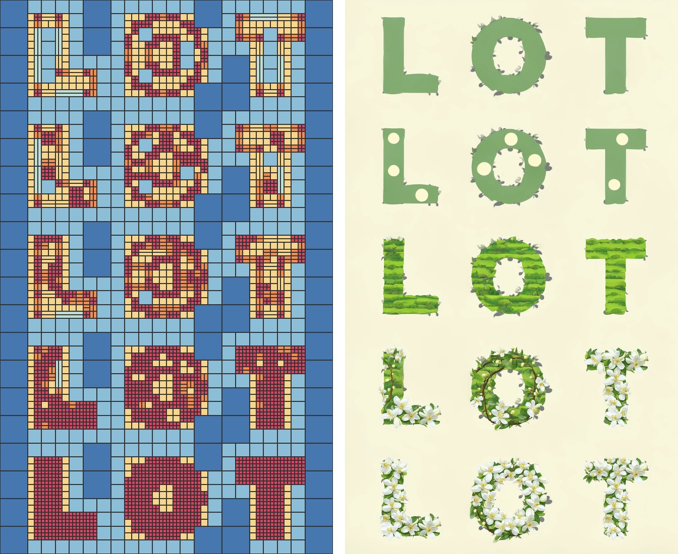
Counting that list was useful. 4,120 tokens tile all 15,360 cells, a 3.73× compression. The 1×1 tokens are 69% of the sequence but cover only 18% of the image. The 4×4 and 8×8 tokens are 9% of the sequence and cover 61%. That asymmetry is what you are buying: the attention and the MLPs see mostly fine tokens, because most of the image is easy and costs almost nothing. It also contains 162 tokens of 2×1, 152 of 1×2, and a few 8×1 and 1×8 strips, so this is quadtree-like rather than a quadtree. The texture-variance rule coarsens one axis at a time along edges.
Where the layout comes from
The model never sees the signal that made the layout. It gets the text prompt and the rectangles, nothing else. Appendix A.3 describes four ways to make the rectangles, and they share one move: turn the signal into "how fine must this spot be", then tile.
Boxes and semantic masks assign a level to each region, mapped to an extent (8, 4, 2, 1). The background gets a coarser level than any selected region, and where regions overlap the finer one wins. Texture variance adapts the variable-rate-shading rule from real-time graphics: a region is coarsened along a direction when the luminance error from doing so stays under a tolerance , which is why it produces strips. Depth goes through a circle-of-confusion model, , so pixels far from the focal plane get large blur radii and large tokens. A region only merges when its smallest blur radius allows it, so one in-focus pixel keeps its block fine.
The fourth source is the one the agent demos use, and the simplest to reason about. Paint a detail map with four brush colours scoring 0, 0.3, 0.6 and 1, average it onto the token lattice, multiply by a gain, clip to . Then start from 8×8 blocks and split a block of extent into four whenever its brightest cell clears a threshold:
That rule, with the real FLUX.2 lattice, is the widget below. The scenes are toys I drew; the split rule, the RoPE centre and the head sizes are the paper's and the model's. The paper doesn't publish its thresholds, so I picked 0.2, 0.45 and 0.75.
a subject box (0.6) with a finer box for the face (1.0); background 0.3
Blocks start at 8x8 and split while the brightest cell under them clears the threshold for their size (0.2, 0.45, 0.75 here). The gain multiplies the whole detail field, so it moves every block at once, which is how the paper exposes the budget for painted maps. Real layouts from texture variance also contain rectangles such as 2x1 and 8x1; this quadtree only makes squares.
Two things stand out once you drag the gain. First, the budget is not a number you type. It is whatever the thresholds and the gain produce, which the paper says outright: the controls "let the user adjust the resulting token count without requiring an exact token budget". Second, the count moves in jumps. A whole region crosses a threshold at once and the sequence length snaps from 772 to 1,954 tokens on my painted scene. A real interface would want a search over the gain to land near a target, and the paper's evaluation instead sweeps VRS thresholds and reports whatever budgets come out (1.52× to 2.94× in the main tables, up to about 8× in the appendix sweep).
Teaching a pretrained DiT to eat rectangles
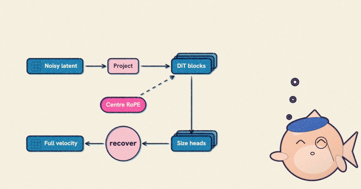
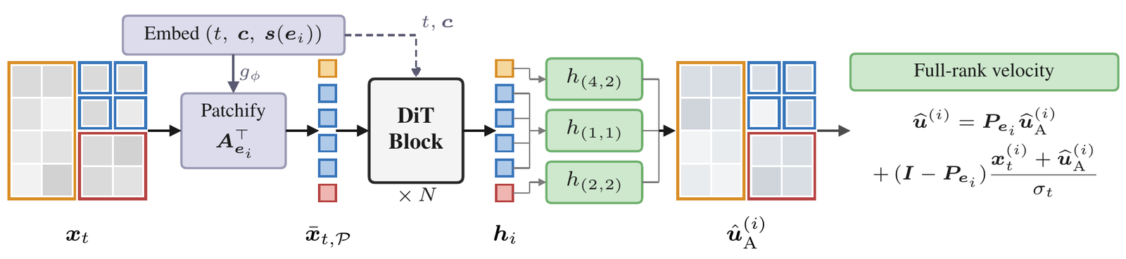
Feeding a DiT a sequence of mixed-size tokens breaks three things at once. The input projection expects 128 numbers per token and an 8×8 token has 8,192. The output head emits one token's worth of velocity and the sampler needs a full-resolution velocity for every latent pixel, because the state being integrated and the VAE decoder both live on the full grid. And RoPE gives each token a grid position but says nothing about how big it is. LoT fixes each with as little new machinery as it can.
The patch lift
For every extent the authors fit a semi-orthonormal matrix , with . For an 8×8 token on FLUX.2 that is 8,192 by 128. A coarse token is the projection of the dense patch underneath it,
The fit is orthogonal Procrustes between dense patches and "extent-matched multi-scale VAE tokens" (Eq. 14). Read that slowly: the target is what the pretrained VAE plus patchify produce when the image is encoded at the coarser scale. So maps a block of fine latent onto something shaped like a lower-resolution latent token, which the pretrained input layer has seen before. The extent's input head starts as the pretrained input projection composed with , so on day one a coarse token embeds like a low-resolution one. That initialisation is where most of the pretrained prior survives.
A scalar per extent fixes the magnitude mismatch (projection does not preserve token norms). AsymFlow handled this by rescaling the timestep. LoT can't, because a sample with mixed extents would then need a different timestep per token while the DiT was trained with one shared . So the authors divide each clean patch by its before adding noise and multiply back before decoding (Eq. 16). Every token keeps the same and the projected noise stays standard Gaussian. Small decision, and the right one: it keeps the conditioning path exactly as pretrained.
Why a coarse token can still return a full velocity
This is the part I had to work through on paper. Flow matching here uses and the target velocity , where is clean data. A coarse token only shows the network , 128 of 8,192 dimensions. It cannot possibly know the noise in the other 8,064.
Asymmetric flow (arXiv 2605.12964, Chen, Ackermann, Kim, Wetzstein and Guibas) changes the target so it doesn't have to. With the projector , the network predicts
the clean patch at full resolution, but the noise only inside the subspace the token can see. The full velocity comes back without the network (Eq. 9):
Check it with the exact target. . For the other part, , and applying kills the term and leaves . Divide by and you get . The two pieces add up to . The unseen noise is never predicted; it is read off the state the sampler already holds, once the clean patch is known.
So the job of a coarse token is to predict a full-resolution clean patch from one hidden vector. Its output head is linear, , initialised as . For an 8×8 token that maps 3,072 numbers to 8,192, so the clean patches it can express live in a subspace of at most 3,072 dimensions. My reading is that this is where the smoothness of coarse regions comes from: the paper describes LoT "favoring smoother or defocused content in coarser-token regions", and a rank-limited linear decoder from one token can only paint so much texture into 64 latent positions. The paper doesn't make this argument; it is mine.
The ablation says how much the asymmetric target carries. Replace the recovery with heads trained to output the full-resolution flow directly ("direct HR prediction"), keep everything else, and FID goes from 13.80 to 26.49 at 1.52× compression and from 13.35 to 68.51 at 2.94×. Nothing else in the paper moves the numbers that much.
Position and size
Each token keeps the pretrained axial RoPE, indexed at its centre on the finest grid (Eq. 13):
An 8×8 token at the corner sits at ; a 1×1 token keeps its integer position, so a layout of all unit tokens is the pretrained model exactly. Fractional positions are free with RoPE, since the rotation is a continuous function of position. If you want the rotation itself from the ground up, the RoPE page covers it. The paper's point is that this is query-independent: unlike the multi-scale RoPE variants in Foveated Diffusion and similar work, no token needs a position map that depends on who is asking, so the attention stays a stock dense kernel.
Size goes in separately: four numbers through a zero-initialised MLP, added to the token embedding. Zero init means it starts as a no-op. It matters less than I expected. Turning it off costs FID 13.80 to 14.58 at 1.52× compression and 13.35 to 14.93 at 2.94×, small next to the other ablations. The extent-specific input and output heads already tell the network a lot about size.
None of the code is public, so I wrote the forward pass out from Eqs. 7 to 13 to make the shapes concrete. It is my sketch, not the authors' code:
# my sketch of one LoT denoising call (not released code); FLUX.2 klein 4B shapes
# x_t: (H0, W0, 32) noisy latent in the scaled space; layout: list of (u, v, eh, ew)
tokens, pos, shape = [], [], []
for (u, v, eh, ew) in layout:
    patch = patchify(x_t)[u:u+eh, v:v+ew].reshape(-1)        # eh*ew*128 numbers
    z = A[(eh, ew)].T @ patch                                # 128, Eq. 7
    tokens.append(W_in[(eh, ew)] @ z + g_phi(s(eh, ew)))     # 3072, Eq. 12
    pos.append((u + (eh - 1) / 2, v + (ew - 1) / 2))         # RoPE centre, Eq. 13
h = dit_blocks(tokens, rope=pos, t=t, text=c)                # L tokens instead of 4,096
u_hat = empty_like(x_t)
for (u, v, eh, ew), hi in zip(layout, h):
    ua = head[(eh, ew)](hi)                                  # eh*ew*128, Eq. 10
    P = A[(eh, ew)] @ A[(eh, ew)].T
    xt = patchify(x_t)[u:u+eh, v:v+ew].reshape(-1)
    full = P @ ua + (I - P) @ (xt + ua) / max(sigma_t, 1e-6) # Eq. 9
    write_patch(u_hat, u, v, eh, ew, full)
x_next = x_t + dt * u_hat                                    # ODE step on the full grid
In practice you would batch the patches by extent and never build as an 8,192-square matrix: costs two thin matmuls. The point of writing it out is the loop structure. The transformer runs on tokens; everything before and after it is per-patch linear algebra on the full grid, and that part does not shrink.
Training is a LoRA, not a new model
The image model is FLUX.2 klein base 4B with its text encoder and VAE frozen. The per-extent input and output heads, the shape MLP and the final adaptive norm are trained in full; the attention, MLP and timestep layers get rank-256 LoRA adapters. 50,000 steps at batch 32, AdamW at 1e-4, on Aesthetic-Train-V2 at 1024×1024 with a 95/5 split, and each training image gets layouts from SAM 3 masks and boxes, texture variance and a depth estimator. The loss is a clean-data MSE weighted by , with power-function EMA () for evaluation.
A 9B variant trained separately on three million LAION images, 32 H100s, batch 256, and the qualitative demos use its 24,500-step EMA checkpoint. The video model is Wan2.1 T2V 14B, 4,000 steps at batch 32 on 81-frame 1280×720 clips from Vchitect's dataset, with the layout mix 50% masks or boxes, 25% texture variance, 25% depth of field. Its grids are capped at 3,072 tokens per latent time slice to avoid running out of memory. Wan's dense slice at 720p is 45×80 = 3,600 tokens, so every training clip was compressed at least a little; I'd like to know how the model behaves at full density, and the paper doesn't say.
The cheapness is the attraction. These are fine-tunes of open checkpoints, and the method touches the model in four places: the heads, a small MLP, the RoPE index and LoRA. If code appears, it would be a modest job to port to another flow DiT.
Where the time goes
Now the speed. The image numbers come from Table 1 plus the extra budget in Table 5, all on an H100 at 30 steps, timed from prompt encoding to VAE decode:
| token compression | LoT time | LoT speedup | ratio |
|---|---|---|---|
| 1.00× (dense control) | 5.77 s | 1.00× | |
| 1.52× | 4.37 s | 1.32× | 0.87 |
| 1.89× | 3.70 s | 1.56× | 0.82 |
| 2.41× | 3.18 s | 1.82× | 0.76 |
| 2.94× | 2.83 s | 2.04× | 0.70 |
The last column is speedup divided by compression, and it falls as compression rises. I fitted to the dense reference (5.7783 s) and the four LoT timings: s, s, with every residual under 0.09 s. Read as the work that doesn't shrink with the token count: text encoding, the VAE decode, the per-patch recovery on the full grid, launch overhead. It is about 23% of a dense image, and it caps the speedup near 5.8/1.33, about 4.4×, however coarse the layout gets.
The video table goes the other way. At 2×, 2.5× and 3× compression LoT-Wan2.1 runs 2.26×, 2.91× and 3.53× faster. Speedup beats compression at every budget, and so does every baseline's.
Sequence length explains both. Per token and per block, the linear layers cost a fixed amount while attention costs something proportional to the sequence length. My rough count from the configs, ignoring text tokens and fixed costs: on FLUX.2 klein 4B (width 3,072, MLP ratio 3) a token's linear layers cost about 189 MFLOPs per block and its attention about 50 MFLOPs at 4,096 tokens, so attention is roughly a fifth of the block and the block cost falls about linearly with the token count. On Wan2.1 14B (width 5,120, FFN 13,824), a 720p, 81-frame clip is 21×45×80 = 75,600 tokens; linear layers are about 493 MFLOPs per token and attention about 1,548. Attention is three quarters of the work, and it shrinks with the square of the token cut.
The project page's own timing file fits the same pattern. Its five bounding-box demos run the 9B model at 1536×1024, 6,144 dense tokens, 50 steps: 28.7 s dense against 11.5 to 14.9 s for LoT, which works out to 1.93× to 2.49× for 2.32× to 3.15× fewer tokens. The teaser image goes 2.5× faster for 2.16× fewer tokens, and Wetzstein's thread puts its dense count at 14,336. Longer sequences, better ratio.
Left: the dashed diagonal is speedup equal to compression. Image points sit below it, video points above it. Right: the dashed horizontal line is the dense model fine-tuned on the same data. Every method at a given budget gets the same layout, derived from a reference image or a reference video.
The abstract promises "significant speedups determined by the layout's token budget". True, with a footnote that matters for deployment. At 1024² on a 4B model, half the tokens buys you about 1.6×. On long video, or images well past 1024², the same layout buys more than its token count. If I were picking where to try this first, it would be video.
Reading the comparison tables carefully
Table 1 is where LoT looks best, and it is worth knowing what it measures. All methods are evaluated on the 5,261 held-out prompts, and for each prompt the layout is derived by texture variance from that prompt's held-out reference image. The paper is upfront that this "is a layout-conditioned comparison: the layout provides reference-derived spatial detail allocation beyond the text prompt". The generator never sees the reference pixels, but it is told where the reference image has texture.
That explains the most striking row. The dense control, FLUX.2 4B fine-tuned on the same split for the same 20,000 steps, scores FID 16.75. LoT at 1.89× fewer tokens scores 13.36. A model with fewer tokens beats the dense model on fidelity to the reference set, and on pFID and TOPIQ too. Appendix Figure 14 sharpens it. LoT's FID is U-shaped in compression, higher near 1.2× than around 3×, where it bottoms out, then climbing again toward 8×. I read both as the layout carrying information about the test images rather than as coarse tokens making better pictures. On the learned human-preference scores, which don't look at the reference set, LoT falls steadily below the dense model as the budget shrinks: HPSv3 10.43 dense, 10.12, 9.75, 9.55; ImageReward 0.95, 0.88, 0.85, 0.83. Those scores are the honest cost curve, and it is a gentle one.
Against the other token-reduction methods the picture is cleaner, because they get the same layouts and the same 20,000-step fine-tune (except ToMe-SD, which is training-free). LoT has the best HPSv2.1, HPSv3, FID, pFID, TOPIQ and MUSIQ at every budget, and is the fastest at every budget, though only just ahead of ToMe-SD (1.56× against 1.54× at the first budget). ToMe-SD collapses on quality: HPSv3 0.93 at 2.94×. The only place LoT loses is ImageReward at the first budget, where DDiT's 0.885 edges its 0.883.
Two caveats on the baselines. DDiT and Foveated Diffusion were extended by the authors to support 8×8 tokens, so their numbers are for ports, not their original code. And Foveated Diffusion, the same group's earlier mixed-resolution method, runs only 1.04× to 1.18× faster than dense in this table despite the same token cuts. That looks to me like an implementation cost (its query-dependent position maps) more than a ceiling of the idea, but the paper doesn't analyse it.
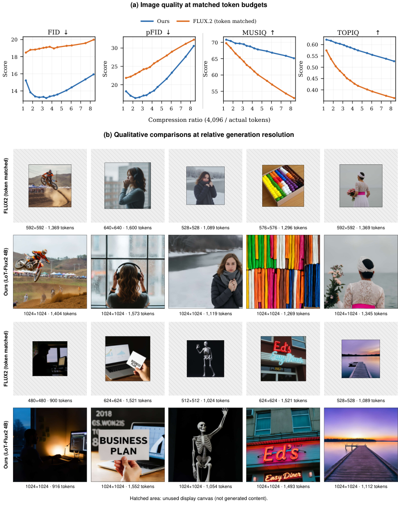
The most useful baseline in the whole paper is in that appendix figure, and it is the boring one: pretrained FLUX.2 run at a lower resolution with a token count matched per image, then bicubically upsampled. Against that, LoT's MUSIQ falls from about 71 to 65 across the sweep while the low-resolution baseline falls from 70 to 53. If your alternative to LoT is "render smaller and upscale", LoT wins and the gap widens with compression. I'd have liked MrFlow-style resolution climbing in the same chart, since it attacks the same budget from the time axis and the paper says the two are compatible.
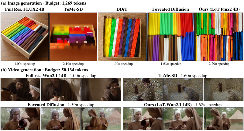
The video table follows the same shape on the two VBench scores that track appearance. Imaging quality is 0.647 dense and 0.612, 0.585, 0.565 for LoT at 2×, 2.5× and 3×; Foveated Diffusion is lower at each, ToMe-SD much lower. On the temporal scores LoT is level with Foveated Diffusion and slightly below dense. The evaluation layouts here come from reference videos generated by a different model (MiniMax-H3), because the held-out clips "were mostly static". Fair enough, and a reminder that the layouts in every table are oracle-ish: they describe where detail ended up in some real or generated video, not a guess made from the prompt.
The layout also moves the subject
Appendix A.9 runs an experiment that changed how I think about the method. Take 2,096 COCO prompts with one clear subject. Build a layout with 1×1 tokens inside the subject's real box and 2×2 outside, then a second layout with the same box translated somewhere else. Same prompt, same noise, same token count. The subject follows the fine tokens: the share of the detected subject inside the target box is 61.17% for LoT-FLUX.2 4B against 45.38% for dense FLUX.2, and 66.83% against 44.94% at 9B.
The authors present this as controllability, and it is. It is also a warning. A LoT layout is not a neutral compute hint; the model has learned that fine tokens are where things go. If you feed it a layout that disagrees with the prompt, it will bend the picture toward the layout. In the agent and storyboard settings the paper is aimed at, where a planner draws the layout and the layout is the intent, that is a feature. As a drop-in accelerator for arbitrary prompts, you need a layout source you trust, and the paper does not test one that is predicted from the prompt alone.
Where it breaks
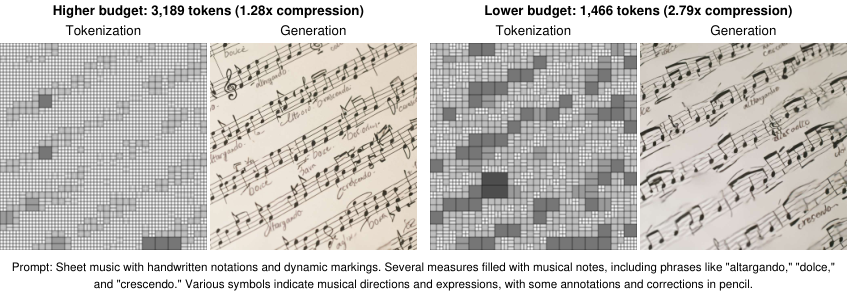
The paper's own limitation figure is the one I would have asked for. Sheet music is fine structure everywhere. At 3,189 tokens (1.28× compression) the staff lines hold; at 1,466 tokens (2.79×) they fragment and bend. There is nothing to save when every region is hard, and forcing a budget anyway breaks structure first. Thin, long, regular things like text lines, cables and fences are what I'd expect a rank-limited coarse token to struggle with too, though the paper only shows the sheet music.
A few smaller things I could not reconcile. The text says LoT-FLUX.2 achieves "1.32–2.04×" speedup in Table 1, but Table 1's lowest LoT speedup is 1.560×; 1.32 is the 1.52× budget that appears only in the ablation table. The video range is given as "1.58–3.53×", and I could not find 1.58 in any video table; the lowest in Table 2 is 2.262×. Wetzstein's thread mentions "up to 4.6× when detail is more concentrated", which no table in the paper reports. The typography gallery on the project page labels its outputs "LoT-Flux.2-14B" and "Full-resolution Flux.2-14B", a size the paper never mentions; the 4B and 9B are the only models it describes. None of these change the story, but they are the kind of thing a code release would settle.
Would I use it
The core idea is right and overdue. Generation pipelines are growing a planning stage, and that stage already knows where detail goes; letting it set the compute is cleaner than having the DiT rediscover it every step through attention scores or similarity merges. LoT does it with almost no new architecture, and the asymmetric-flow recovery is the piece I would reuse first, because it answers the question every coarse-token method has to answer (how do you get a full-resolution velocity out of fewer tokens) with algebra instead of a decoder.
For 1024² images on a 4B model, the speed is real but modest, about 1.6× at half the tokens, and the fixed cost puts a ceiling near 4.4×. For long video it is better than linear. The quality cost on preference scores is small and smaller than any baseline's. The two things I would check before trusting it in a product are what happens with a layout predicted from the prompt alone, and how far the layout pulls content you didn't ask for. Neither is measurable until the weights are out. The neighbours on this site attack the same budget elsewhere: Sana shrinks the token grid with a deeper autoencoder, PixelUMM and PixelDense drop the VAE altogether, and Mixture-of-Depths is the language-model cousin where a router picks which tokens a block computes. For the DiT itself, start at the Diffusion Transformer page; FLUX 3 is where the FLUX line went next.
How I checked
I read the paper and its appendix from the arXiv HTML (v1, 5 October 2026), and the X threads by Brian Chao and Gordon Wetzstein through the fxtwitter mirror. I shallow-cloned the project page's repository, georgenakayama/lotdiffusion at commit 5edcc89, which holds no model code. From it I counted the flowering-letters layout in layout-inspector-data.js (4,120 rectangles covering 15,360 cells, per-extent counts and per-fifth counts), rendered that layout for the figure above, and read supplementary/bbox_timings.json and bbox_examples.json for the 9B timings and token counts. Model shapes come from the published configs: FLUX.2 klein base 4B (in_channels 128, 24 heads of 128, 5 double-stream and 20 single-stream blocks, MLP ratio 3) and Wan2.1 T2V 14B (width 5,120, FFN 13,824, 40 layers, patch 1×2×2, 16 latent channels).
The speed-to-compression ratios, the fit and its 4.4× ceiling, and the per-token FLOP split are my arithmetic on the paper's tables and those configs. The FLOP split ignores text tokens, the double-stream blocks' separate text weights and kernel efficiency, so treat it as a direction, not a prediction. I checked the Eq. 9 recovery by hand. The idea that rank-limited coarse heads explain smooth coarse regions is my reading, not the paper's. I could not run anything: no code or weights have been released.