2026-08-26 · 24 min · diffusion · linear-attention · autoencoders · distillation · nvidia
A 1:53 narrated explainer, drawn in code. Every number and picture in it is this article's own; the sources are below.
› transcript
Hi, I'm Tortilla! Sana is known as the linear-attention image model. But its bigger trick happens before attention even runs. Here's how it works. Sana's autoencoder compresses thirty-two times per side, with patch size one. So the transformer sees four times fewer tokens, before any attention runs. A diffusion transformer works on an autoencoder's latents. FLUX and SD3 shrink each side eight times, then patch by two: a 1024 pixel image becomes 4096 tokens. Sana's autoencoder shrinks each side thirty-two times, with no patching on top. The same image is a thirty-two by thirty-two grid: 1024 tokens. The transformer denoises that grid. Its self-attention is linear, so cost grows with the token count, not its square. The prompt goes through Gemma, a small language model with its head removed. The transformer reads it through ordinary softmax cross-attention. Softmax attention builds a token-by-token matrix. Swap the exponential for a ReLU, and you can multiply in a different order. Keys times values first. That's a small thirty-two by thirty-two state, the same size at every resolution. Then each query reads that state, so the cost is linear in the number of tokens. Given the autoencoder, linear attention buys one point one two times at ten twenty-four pixels, and three at forty ninety-six. The autoencoder always buys about four. At every resolution Sana ships, the autoencoder is the bigger lever. Linear attention is insurance against the resolution going up. To recap: compress harder before the transformer, keep attention's state small, and know where each lever pays. Every source is in the full article. I'm Tortilla. Bye!
Why read this
Essentialtop 10%Rebuilds Sana's FLOP table from its configs to show the 32x autoencoder, not linear attention, carries the speedup below 5000px, and that 100x is a 4K figure.
- Original, source-checked analysis
- Interactive explanations
- Runs on a consumer GPU
Image & video generationMixed licencesPractitioner model
How this was scored
- Is it new?
- 2 of 3: A real new idea, method or capability
- Can I trust it?
- 3 of 3: Reproduces the headline result, or shows from primary files it is wrong
- Can I run it?
- 2 of 3: Open code or weights with real limits
- Will I understand it?
- 3 of 3: Mechanism carried by interactives built from real code or data
- Can I act on it?
- 2 of 3: A concrete recipe, numbers or comparison
- Will it last?
- 2 of 3: A reference for a year or more
- Does it affect many?
- 2 of 3: A widely used model, tool or lab release
- Only here?
- 3 of 3: The only place this analysis exists
Score 84 of 100, ranked 9 of 577 rated articles. Each question is answered 0–3 by hand, and a 3 is rare. How articles are scored
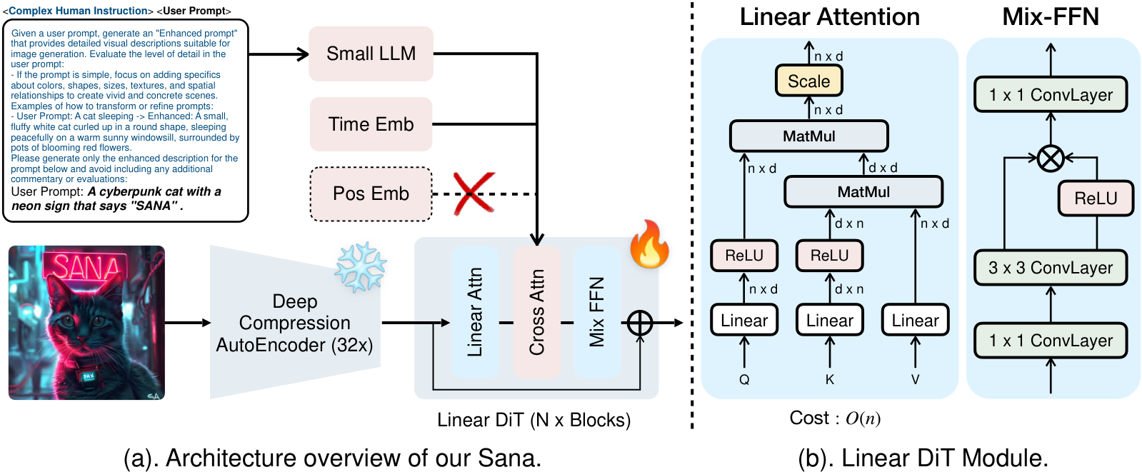
Sana is usually introduced as the linear-attention image model. The paper is titled Efficient High-Resolution Image Synthesis with Linear Diffusion Transformer; the repo's own summary leads with "Linear Attention: Replace vanilla attention in DiT with linear attention for efficiency at high resolutions"; the headline is 20× smaller and 100× faster than FLUX-12B.
I cloned NVlabs/Sana at commit 5498e5b and read the parts that
would have to be true for that story to hold: diffusion/model/nets/sana_blocks.py where the linear
attention lives, the YAML configs that define every released checkpoint, the DC-AE model zoo, and
train_scripts/train_scm_ladd.py where Sana-Sprint gets distilled. Then I rebuilt the paper's own
FLOP accounting from those configs.
The linear attention is real and it is nicely implemented. It is also the second-largest thing Sana does — at 512px, at 1024px, at 2048px and, by a narrowing margin, at 4096px. The largest is an autoencoder that throws away four times more tokens than the one FLUX and SD3 use, before the transformer has started.
| What it is | NVlabs/Sana at 5498e5b — an efficiency-first family of image and video diffusion models with full training + inference code |
| Actually in this tree today | Sana 1.0, Sana-1.5, Sana-Sprint, SANA-Video / LongSANA, SANA-WM, SANA-Streaming, Sol-RL configs |
| Not in this tree | Sol-Engine — the README's newest headline (3.95× on GB200) lives on a separate sol-engine branch |
| Image DiT | SanaMS_600M_P1_D28 = 28 layers × 1152 · SanaMS_1600M_P1_D20 = 20 × 2240 · SanaMS_4800M_P1_D60 = 60 × 2240 |
| Self-attention | LiteLA — ReLU-kernel linear attention, 70 heads of dim 32 at hidden 2240 |
| Cross-attention | softmax, xformers memory_efficient_attention, 20 heads of dim 112 |
| Tokenizer | DC-AE-F32C32 — 32× spatial downsample, 32 latent channels, DiT patch size 1 |
| Text encoder | Gemma-2-2B-IT with the LM head stripped (.get_decoder()), caption_channels: 2304 |
| Positional encoding | none at 512/1024px (use_pe: false); sincos with interpolation at 2K/4K |
| Sampling | flow matching, flow_shift: 3.0, Flow-DPM-Solver, 20 steps · Sprint: TrigFlow + sCM + LADD, 1–4 steps |
| Licence | code Apache-2.0; released weights also Apache-2.0 — but the bundled text encoder is Gemma |
| Stack | Python ≥ 3.11, torch 2.9.1 / cu128, xformers 0.0.33 |
Two levers, and only one of them is the famous one
Every latent diffusion model has a token count it never gets to argue with. An autoencoder with downsample factor maps an image to latents, and the DiT then groups those into patches, so the transformer sees
tokens. PixArt, SD3 and FLUX all use with : an effective stride of 16, so a 1024px image is 4096 tokens. Sana's configs say something different:
# configs/sana_config/1024ms/Sana_1600M_img1024.yaml
model:
  model: SanaMS_1600M_P1_D20   # patch_size = 1
vae:
  vae_type: AutoencoderDC
  vae_pretrained: mit-han-lab/dc-ae-f32c32-sana-1.1-diffusers
  vae_latent_dim: 32
vae_downsample_rate: 32, : an effective stride of 32, so the same image is 1024 tokens. That is four times fewer before any attention runs, and the paper is explicit about why it prefers spending the compression in the autoencoder rather than the patchifier — the AE should "take full responsibility for compression, allowing the latent diffusion models to focus solely on denoising."
The second lever is what happens to those tokens. Softmax self-attention costs ; Sana's
LiteLA costs . The two levers multiply, and the interesting part is that they multiply
unevenly — drag the resolution and watch which one is carrying the load:
The cleanest way to read it is marginally: given the other lever, what does each one still buy? The autoencoder always buys the same thing — 4× fewer tokens, so asymptotically a flat 4× — and linear attention buys 1.02× at 512px, 1.12× at 1024px, 1.50× at 2048px and 3.01× at 4096px. It does not overtake the autoencoder until about 5000px, roughly 25,000 tokens. Every resolution Sana ships at is on the wrong side of that line.
The combined numbers are still large, because they compound: 5.8× at 1024px and 36× at 4096px against an f8/patch-2 softmax DiT of identical width and depth. But the split matters if you are deciding what to copy.
This is not my reinterpretation of the paper. It is the paper's own Table 8, which ablates the block design at 1024px on an A100:
| Blocks | AE | MACs (T) | Throughput (/s) | Latency (ms) |
|---|---|---|---|---|
| FullAttn & FFN | F8C4P2 | 6.48 | 0.49 | 2250 |
| + LinearAttn | F8C4P2 | 4.30 | 0.52 | 1931 |
| + MixFFN | F8C4P2 | 4.19 | 0.46 | 2425 |
| + Kernel Fusion | F8C4P2 | 4.19 | 0.53 | 2139 |
| LinearAttn & MixFFN | F32C32P1 | 1.08 | 1.75 | 826 |
| + Kernel Fusion | F32C32P1 | 1.08 | 2.06 | 748 |
Read the latency column. Swapping softmax for linear attention takes 2250 ms to 1931 ms. Adding Mix-FFN — which the paper needs, because linear attention alone converges badly — takes it back up to 2425 ms, slower than the softmax baseline it replaced. Triton kernel fusion claws it back to 2139 ms. Then the autoencoder changes, and the same fused linear block runs in 748 ms. The whole block redesign is worth 1.05×; the tokenizer swap on top of it is worth 2.9×.
I wanted to be sure I was reading the columns right, so I rebuilt them. Take the 0.6B config as the
repo defines it — depth 28, hidden 1152, mlp_ratio: 2.5 Mix-FFN, linear_head_dim: 32, 300 text
tokens — and count multiply-accumulates from the shapes:
softmax self-attn   2 N² d               LiteLA    2 N d (d_h + 1)
MLP-FFN (ratio 4)   8 N d²               Mix-FFN   N (7.5 d² + 22.5 d)
qkv + out proj      4 N d²
cross-attn          2 N d² + 2 N Lt d + 2 Lt d²
Doubling for FLOPs and multiplying by 28 layers reproduces 6.48 / 4.30 / 4.19 / 1.08 as 6.63 / 4.48 / 4.34 / 1.12 — every row within 4.2%, which is about what the adaLN and norm terms I skipped are worth. The column is FLOPs rather than MACs despite the header, and it is the 0.6B model. The arithmetic is otherwise exactly what the configs say it should be.
What LiteLA actually computes
The kernel is a dozen lines and worth reading in full, because the trick is in a padding call.
# diffusion/model/nets/sana_blocks.py — LiteLA.attn_matmul
def attn_matmul(self, q, k, v: torch.Tensor) -> torch.Tensor:
    q = self.kernel_func(q)          # nn.ReLU
    k = self.kernel_func(k)
    v = F.pad(v, (0, 0, 0, 1), mode="constant", value=LiteLA.PAD_VAL)  # PAD_VAL = 1
    vk = torch.matmul(v, k)
    out = torch.matmul(vk, q)
    out = out.float()
    out = out[:, :, :-1] / (out[:, :, -1:] + self.eps)
    return out
Softmax attention computes , and the in the middle is an matrix. Replace the exponential with a feature map and it becomes , which associativity lets you rebracket as — and now the inner product is , independent of . Sana uses .
The padding is how the denominator rides along. Attention has to normalise by , which is a different contraction from the numerator. Appending a row of ones to makes the last row of the state exactly that sum, so one matmul produces numerator and denominator together and the final line divides them. It costs one extra row of a 32×32 matrix.
That state is the whole memory of the layer, and it is the same size at every resolution:
Two things fall out that the paper's prose does not dwell on. The first is the rank bound: the attention map LiteLA implies is , a product of an and a matrix, so it has rank at most 32 no matter how many tokens there are. At 4096px that is 16,384 tokens mixed through a rank-32 map.
The second is that a ReLU kernel has no temperature. ReLU-then-normalise is homogeneous of degree
zero, so scaling the query changes nothing at all; softmax's exponential means the same scaling is
exactly the knob that sharpens attention to a hard argmax. Slide in the widget and only one
row moves. Sana's compensation is architectural rather than attentional — the 3×3 depthwise
convolution inside Mix-FFN puts local mixing back — and the paper is honest that without it,
"linear attention models suffer from much slower convergence."
Two more things I did not expect to find in the source.
The cross-attention is not linear. SanaMSBlock dispatches attn_type to LiteLA, but every
cross_attn_type except vanilla lands on MultiHeadCrossAttention, which calls
xformers.ops.memory_efficient_attention. Sana is a linear self-attention DiT; conditioning on the
text stays softmax. That is the right call — cross-attention is , already
linear in — but "Linear DiT" describes one of the two attention operators in the block.
Every config sets fp32_attention: true, and the kernel force-casts to float before dividing.
This is not paranoia. Softmax is self-normalising; a ReLU kernel is not, so the accumulated numerator
and denominator have no bound. Sana-1.5 reports the failure mode directly: the ReLU-linear attention
logits "grow uncontrollably and frequently exceed the numerical range of FP16," which is why every
1.5 and Sprint config turns on qk_norm: true and cross_norm: true. (The paper puts FP16's ceiling
at 6.5e5; it is 65,504. The mechanism is right, the constant is a decimal place off.)
The autoencoder, and what 32× costs
DC-AE-F32C32 is six stages of encoder — width_list=[128,256,512,512,1024,1024], the last three
EViTS5_GLU blocks — giving five 2× downsamples, and 32 latent channels. Per image element that is
compression against the f8c4 VAE's ; per token, which is what the
transformer actually pays for, it is 4× fewer.
Compression that aggressive used to be a known-bad idea. The paper's Table 1 is the rebuttal, on MJHQ-30K:
| Autoencoder | rFID ↓ | PSNR ↑ | SSIM ↑ | LPIPS ↓ |
|---|---|---|---|---|
| F8C4 (SDXL) | 0.31 | 31.41 | 0.88 | 0.04 |
| F32C64 (SD) | 0.82 | 27.17 | 0.79 | 0.09 |
| F32C32 (Sana) | 0.34 | 29.29 | 0.84 | 0.05 |
The earlier F32 attempt was two and a half times worse on rFID than f8c4; this one is within 0.03. PSNR is still 2 dB down, which is a real gap and shows up as softness in fine texture — but the argument is that a 2 dB reconstruction penalty is a good trade for a 4× cheaper transformer, and the generation FID numbers support it. There is a companion ablation worth flagging: F8C16P4, F16C32P2 and F32C32P1 all produce the same 32×32 token grid at 1024px, F8C16 reconstructs best, and F32C32P1 generates best. Where you put the compression matters more than how much reconstruction error it costs.
The channel count is a similar trade: C=16 converges fastest but reconstructs worse, C=64
reconstructs best but the downstream DiT converges much slower. C=32 is the compromise, and the
scale_factor: 0.41407 in every config is the latent normalisation that goes with it.
No positional embedding, except where there is
The clean surprise in Sana 1.0 is that the DiT has no positional encoding. use_pe: false in the
512px and 1024px configs, and the architecture figure crosses the Pos Emb box out in red. The
justification is that Mix-FFN's zero-padded 3×3 depthwise convolution leaks absolute position
implicitly, which is a known result for convolutional encoders. It also means nothing in the network
assumes a resolution.
Except the released high-resolution models turn it back on:
# configs/sana_config/2048ms/Sana_1600M_img2048_bf16.yaml   configs/sana_config/4096ms/...
use_pe: true
pe_interpolation: 1.        #  → 2.  at 4096px
and the shipped diffusers config for Sana_1600M_4Kpx_BF16_diffusers carries
"interpolation_scale": 2.0 with "sample_size": 128, while the 1024px checkpoint's config has no
interpolation_scale key at all. So
NoPE holds for the models trained at their native resolution and is dropped for the 2K/4K
fine-tunes — which is the honest version of "positional embedding is not required": not required
when you are not extrapolating.
The text encoder is an LLM you are allowed to instruct
Swapping T5-XXL (4.76B) for Gemma-2-2B-IT (2.61B) is the part everyone quotes, and the loading code is blunt about what it does:
# diffusion/model/builder.py
text_encoder = (
    AutoModelForCausalLM.from_pretrained("Efficient-Large-Model/gemma-2-2b-it",
                                         torch_dtype=torch.bfloat16)
    .get_decoder()
    .to(device)
)
Take a causal LM, throw away the LM head, use the decoder stack as a feature extractor.
caption_channels: 2304 in the model config is Gemma-2-2B's hidden size. Table 9 puts the shipped
encoder, Gemma2-2B-IT, at 2614M params and 0.28s against T5-XXL's 4762M and 1.61s — 5.8×
faster for the same 6.1 FID and 0.2 less CLIP. Worth noting that the best FID row in that table,
5.9 at 0.21s, is Gemma-2B-IT — first-generation Gemma, which is not the model any config loads.
But the size is not the point. The point is that a decoder-only model can be given instructions,
and Sana gives it a long one — the chi_prompt block sitting in every single config, telling the
model how to expand a terse prompt into a detailed visual description. What the pipeline does with
it is the part I had not seen described anywhere:
I tokenised the preamble with the Gemma tokenizer shipped alongside the weights: 1057 characters,
208 pieces. So max_length_all = 209 + 300 - 2 = 507, Gemma runs over 507 positions, and then
select_index = [0] + list(range(-self.config.text_encoder.model_max_length + 1, 0))
caption_embs = self.text_encoder(...)[0][:, None][:, :, select_index]
emb_masks    = caption_token.attention_mask[:, select_index]
keeps slot 0 and the last 299. Slot 208 is the final token of the instruction; everything after is the user's prompt and then padding, which the mask zeroes. For the repo's own example prompt the diffusion transformer ends up cross-attending to 13 vectors. The instruction is never handed to the DiT at all — it works entirely through Gemma's causal attention, which has already folded it into the hidden states at the prompt positions.
That is a genuinely elegant piece of design and it is also a free lunch that isn't free: you pay for
a 507-token forward pass of a 2.6B LLM to condition on a twelve-token prompt, and prompts longer than
298 tokens are silently truncated by truncation=True.
Sana-1.5: grow the depth, then buy quality with samples
Sana-1.5 is three separate ideas bolted to the same backbone, and the configs show all three.
Depth growth. SanaMS_4800M_P1_D60 is the 1.6B's 20 blocks turned into 60, initialised from the
smaller model rather than from scratch, with the output projections of both attentions and the final
point-wise conv zero-initialised so each new block starts as an identity map. One detail is a nice
piece of empiricism: appending new blocks after all the pretrained ones failed — the well-learned
features dominated through the skip connections and the new blocks got stuck — so they delete the
last two pretrained blocks first. Reported as reaching the same GenEval with ~60% fewer steps.
CAME-8bit. train.optimizer.type: CAMEWrapper with block-wise 8-bit first moments and 32-bit
second-order statistics, quantising only tensors above 16K parameters in blocks of 2048. For the 1.6B
that is 43 GB against AdamW's 57 GB — a 25% reduction, which is the number in the appendix, not the
~8× the abstract implies (that is the optimizer-state ratio, not total training memory).
Inference-time scaling. Generate candidates, score them with a fine-tuned NVILA-2B verifier, keep the best few. The repo's own doc puts the 4.8B v2 model's GenEval at 81 → 96 with top-4 of 2048, and notes 32 candidates already clears 90. That is a real result and it is also a 2048× compute multiplier on the thing Sana was built to make cheap. And the README's own comparison table has the 1.5 1.6B at 0.82 GenEval against the 4.8B's 0.81 — the 4.8B still wins DPG (84.7 vs 84.5) and CLIP (29.23 vs 29.12), but on the benchmark the paper leads with, three times the parameters and three and a half times the latency buys nothing.
Sana-Sprint: two steps, on an arc
Sana-Sprint distils the flow-matching teacher into a 1–4 step generator by moving to TrigFlow's parameterisation, where the noising process is a spherical interpolation on :
so is pure noise, is the sample, and the SNR at is exactly — the data scale cancels because the noise carries it too. The training loop is continuous-time consistency distillation (sCM) plus a latent adversarial term, and the code is unusually readable:
# train_scripts/train_scm_ladd.py
v_x = torch.cos(t) * torch.sin(t) * dxt_dt / sigma_data
v_t = torch.cos(t) * torch.sin(t)
F_theta, F_theta_grad, logvar = torch.func.jvp(model_wrapper, (x_t / sigma_data, t), (v_x, v_t), has_aux=True)

r = min(1, global_step / config.train.tangent_warmup_steps)          # 4000
g = -torch.cos(t) * torch.cos(t) * (sigma_data * F_theta_minus - dxt_dt)
second_term = -r * (torch.cos(t) * torch.sin(t) * x_t + sigma_data * F_theta_grad)
g = g + second_term

g_norm = torch.linalg.vector_norm(g, dim=(1, 2, 3), keepdim=True)
g = g / (g_norm + 0.1)                                               # tangent normalisation
weight = 1 / (torch.tan(t) * sigma_data)
loss = (weight / torch.exp(logvar)) * (F_theta - F_theta_minus - g) ** 2 + logvar
The Jacobian-vector product is the consistency condition: it measures how the network's output moves
as you slide along the probability-flow trajectory, and the loss asks that movement to match the
teacher's velocity. Three details are load-bearing. The tangent is normalised to unit length plus a
constant 0.1, which is what keeps sCM from exploding. logvar is a learned per-sample uncertainty
that reweights the loss — the + logvar term is the price for down-weighting. And
cross_attn_type: vanilla in every Sprint config exists for a mundane plumbing reason: the paper
notes PyTorch has no FlashAttention JVP kernel, and the xformers path Sana normally uses for
cross-attention is in the same position, so Sprint swaps in a hand-rolled
scaled_dot_product_attention that is differentiable twice. The source comment says so outright —
# Cast for sCM, right above a cast of q, k and v to fp32.
On top of that sits LADD: a hinge-loss discriminator with heads on blocks [2, 8, 14, 19] of the
frozen teacher, adv_lambda: 0.5 against scm_lambda: 1. And a weighting trick — with probability
0.5 the generator is trained at exactly largest_timestep: 1.57080, pure noise, which is what makes
one-step generation work at all.
Then the inference schedule, where the repo and the paper part company:
SCMScheduler.set_timesteps only honours intermediate_timesteps when num_inference_steps == 2.
Ask for four and it prints a warning, discards the value, and falls back to
linspace(1.5708, 0, 5). The paper's Table 7 gives a searched 4-step schedule of
[arctan(400), 1.3, 1.1, 0.6, 0], which spends three of four steps above — far more of the
budget in the high-noise regime than a uniform split. Both are reachable; only one is the default.
Where the 0.1 seconds actually goes
The Sprint headline is "0.1s per 1024px image on H100." The paper's own Figure 1 breaks it down, and the breakdown is more interesting than the number:
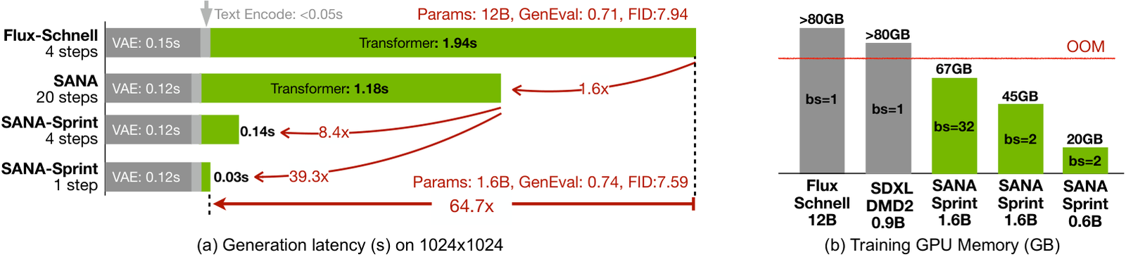
At one step the transformer costs 0.03s and the autoencoder costs 0.12s — the decoder is now four
times the cost of the denoiser. The 64.7× speedup annotated across the bottom is explicitly "the
ratio calculated based on Transformer latency," which is a fair thing to measure and not the thing a
user experiences. End to end on an A100 the paper's own table gives 0.21s for the 0.6B at one
step, and the repo's docs/sana_sprint.md gives 0.24s and 0.25s at two steps for the 1.6B and 0.6B.
So where does 0.1s on H100 come from? 0.12s of VAE decode alone would blow the budget on an A100. The answer is in the Callout above: DC-AE-Lite drops decode to 0.06s and compiling it to 0.03s, and the Lite decoder landed in the repo in August 2025, five months after the Sprint paper. The claim is reachable — newer hardware plus the newer decoder — but the "0.1s" and the paper's own Figure 1 are not describing the same configuration, and nothing in the repo measures the combination. Worth knowing if you are budgeting a latency SLO.
The 100×, checked
The number in the README's first paragraph is "20× smaller and 100× faster than Flux-12B." The first half is arithmetic — 0.6B against 12B — and the second half is defensible but load-bearing about where.
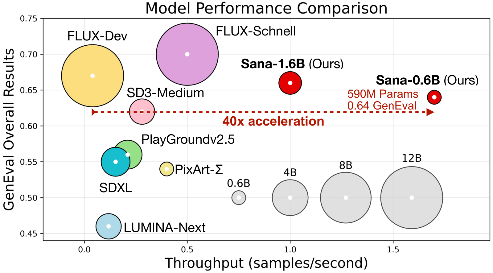
The paper's Table 14 measures four resolutions on an A100 in FP16, batch 16 for throughput and batch 1 for latency:
| Resolution | Sana-0.6B throughput | FLUX-dev throughput | Speedup |
|---|---|---|---|
| 512×512 | 6.67 /s | 0.15 /s | 44.5× |
| 1024×1024 | 1.72 /s | 0.04 /s | 43.0× |
| 2048×2048 | 0.43 /s | 0.008 /s | 53.8× |
| 4096×4096 | 0.104 /s | 0.001 /s | 104.0× |
So: 100× is real, at 4K, on throughput, against FLUX-dev on an A100. At 1024px it is 43× in this table, 40× in the figure, "39×" in the body text and 39.5× in the README's table — four numbers for the same comparison, all in the same repo. None of them is wrong enough to matter, but if you are quoting one, quote the resolution with it.
One thing in that table does not survive a second look. The batch-1 latency column has Sana-0.6B at 0.8s and Sana-1.6B at 0.6s for 512px, and 9.6s versus 5.9s at 4096px — the 2.7×-larger model reported as faster at two of the four resolutions, while being correctly slower at the other two. The throughput column is monotone. I cannot reconcile it; my guess is different tiling or offload settings between rows at 4K, but the table does not say.
Licences, precisely
NVIDIA research releases are usually non-commercial, so I checked rather than assumed.
- The repo is Apache-2.0 (
LICENSE, "Copyright 2024 Nvidia"). The README dates the change to Apache-2.0 at 2025-01-11, three months after release. - The weights are Apache-2.0 too. I pulled the
LICENSEfile out ofEfficient-Large-Model/Sana_1600M_1024px_BF16_diffusers,SANA1.5_4.8B_1024px_diffusersandSana_Sprint_1.6B_1024px_diffusers— all three are the Apache text, and the model-card metadata agrees. This is unusually permissive and it is the single best reason to reach for Sana over a research-licensed alternative. - The autoencoder —
mit-han-lab/dc-ae-f32c32-sana-1.1-diffusers— is MIT. - The text encoder is not Apache. Every diffusers bundle ships
text_encoder/weights whoseconfig.jsonreads"_name_or_path": "google/gemma-2-2b-it", and Gemma is distributed under the Gemma Terms of Use. So the model is Apache-2.0 and the pipeline you actually run is not uniformly so. If that matters to you, it is a swap you have to plan for, not a footnote.
The ledger
What is genuinely new here. Pushing latent compression to F32 with patch size 1 and showing it does not break generation — that is the contribution, and it is the one the rest of the field absorbed. The Complex Human Instruction mechanism is the other: using a causal LM's own in-context behaviour as a prompt enhancer, then slicing the instruction back out of the conditioning, gets the benefit of prompt rewriting with none of the second generation pass. And Sprint's sCM+LADD recipe producing one model that works at 1, 2 and 4 steps — rather than a model per step count — is a real convenience that DMD-style distillations mostly do not offer.
What is convergent. ReLU linear attention is EfficientViT's, applied to a new domain. TrigFlow and sCM are OpenAI's. LADD is Stability's. Depth growth and zero-initialised residual blocks are standard LLM scaling technique. The synthesis is the work, and the repo is honest about the lineage in its acknowledgements.
What I would keep an eye on. The two findings above are the same finding seen twice. Linear attention does not pay for itself until roughly 25,000 tokens, and it costs a rank-32 ceiling on the mixing map — so an image model that never exceeds 16,384 tokens is paying the expressiveness bill without collecting much of the compute refund, and the autoencoder has to carry the efficiency story. A video model is on the other side of both lines: sequences are an order of magnitude longer, so the refund is large, and the quality cost is severe enough that you cannot just eat it. The family's own trajectory says exactly this. SANA-Video 2.0 abandons pure linear attention for a 3:1 hybrid with periodic softmax anchors, and SANA-WM and SANA-Streaming are both titled "Hybrid" too. That is the conclusion the LLM world reached about linear attention, arrived at independently and from the other direction.
And the thing that would change my read. Almost every number above is A100/FP16 from the papers.
The repo ships thorough quality tooling — tools/metrics/ covers FID, CLIP score, GenEval, DPG-Bench
and ImageReward — and nothing at all that reproduces the throughput and latency columns; grepping the
whole tree for either word turns up no benchmark script. The newest performance claims in
the README — Sol-Engine's 3.95× on GB200 — point at a branch that is not in main. If these
latencies are load-bearing for you, measure them yourself: the inference code is all here, the
measurement is not.
If you want the compression argument applied to a tokenizer instead of an attention operator, Mage-Flow makes the same bet from the other side. If you want to see why softmax is hard to beat on a modern GPU regardless of its asymptotics, FlashAttention-3 is the counter-argument in kernel form.