2026-10-06 · 26 min · looped-transformers · flow-matching · diffusion · diffusion-transformers · image-generation · inference
Why read this
Notabletop 60%The LiFT target derived as flow matching along depth, its FLOP accounting re-derived, and the 52% headline traced to a 250-step dense baseline.
- Original analysis
- A lasting reference
- A new technique
Image & video generationAPI onlyResearch paper
How this was scored
- Is it new?
- 2 of 3: A real new idea, method or capability
- Can I trust it?
- 2 of 3: Measures key facts from files, code or configs
- Can I run it?
- 1 of 3: API-only, gated or restrictive licence
- Will I understand it?
- 2 of 3: Mechanism from first principles with figures
- Can I act on it?
- 2 of 3: A concrete recipe, numbers or comparison
- Will it last?
- 2 of 3: A reference for a year or more
- Does it affect many?
- 1 of 3: A specialist community
- Only here?
- 2 of 3: A teardown or measurement few others did
Score 62 of 100, ranked 202 of 445 rated articles. Each question is answered 0–3 by hand, and a 3 is rare. How articles are scored
Earlier today this site ran a piece on LOOM and Looped-DiT, two papers about looping a model more than twice. Both push the useful loop count past two, and in both the loop count is something you fix at training time. Running a looped model deeper than it was trained is where they usually break, and the looped transformer page and the Ouro-vs-Huginn ablations show how many design choices sit underneath that.
Then Pedro Curvo and Mohammad Mahdi Derakhshani posted LiFT. One of its checkpoints was trained with 2 loops, and at 16 loops it gets better: FID 17.07 at two, 9.31 at sixteen, same weights, no retraining. Eight times the training depth, and the curve is still going down at the point where every other looped generator I've read about has turned up.
I expected a better normaliser, or a cleverer form of deep supervision. It is neither. LiFT changes one thing: what each loop is asked to predict. The new target turns out to be flow matching again, one level down, along depth instead of time. Once you see that, the extrapolation stops looking like luck.
The paper is arXiv 2610.05538 (University of Amsterdam and TNO). Its code, weights and W&B logs are listed as "Coming Soon". There is a Gradio demo running the L/2 checkpoint next to two dense baselines. So everything below is checked against the paper's equations, its appendix tables and its own FLOP formula, which I re-derived.
Two ways a flow model can spend compute
A flow-matching model is trained on straight lines. Draw noise and a data point , and put a point on the segment between them:
The network regresses with a plain MSE. Because many pairs pass through the same , the best it can do is their average, the marginal velocity . (The CSFM write-up goes deeper on why that average matters.) Sampling integrates the learned field from noise to data. With Euler and steps, each step costs one network call:
So the usual inference knob is . More steps follow the field more faithfully. But an Euler step can only be as good as the velocity it is handed, and once integration error stops being the bottleneck, more steps buy almost nothing. The paper's own dense L/2 shows this: 16.94 at 50 steps, 16.17 at 100, 15.74 at 250. Five times the compute for about one FID point.
A looped network adds a second knob. Inside each call, run the same core times to get a better velocity estimate. The cost model separates cleanly:
The thread puts it as "one axis is time; the other is depth". The paper's motto is "loop in depth, flow in time". The idea is easy to state. The hard part is training a core that keeps improving as grows.
What the network looks like
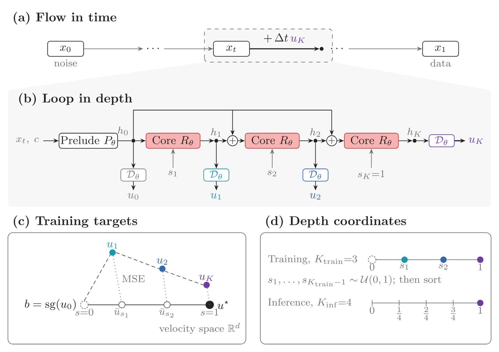
The backbone is an ordinary DiT, split three ways. If you want the DiT itself from the ground up, the Diffusion Transformer architecture page covers patches, adaLN-Zero and the rest. The split, in the paper's Eq. 9:
The prelude is four ordinary DiT blocks that embed the noisy latent once per sampling step. The core is a stack of blocks applied times with the same weights. Each pass normalises the previous state and adds back in, so the input never fades out of the recurrence. The coda is just the prediction head: normalise, modulate, project, unpatchify. It reads out a velocity from any state and does not feed anything back.
Two details carry weight. The conditioning is (time plus class) everywhere, but the core alone also gets , an embedding of a continuous depth coordinate, through the same adaptive-norm and gate machinery DiT uses for time. And the coda has zero transformer blocks. The reason is accounting. Training reads out every state, so a coda with blocks would run times per forward pass. The paper's Eq. 30 puts the extra training cost at . With , what's left is a few prediction heads and depth embeddings. Their Table 17 puts it at 0.0188% of the dense L/2 training budget.
Parameter counts follow the unique blocks. Dense DiT-L/2 is 24 blocks and 457.83M parameters. LiFT-L/2-R10 is 4 prelude blocks plus a 10-block core, 14 unique blocks and 270.24M parameters. Trained with , it executes blocks per forward pass, exactly the dense model's depth. The paper uses this to match training compute within a scale: same executed depth, same 500,000 updates at batch 256, fewer unique weights.
The target, which is the whole paper
The obvious way to train this is to ask every readout to predict . This is deep supervision, what ELT and the Deep Supervision in Looped-DiT do, and its failure is easy to see. If loop 2 is already supposed to output the final answer, loop 3 has no defined job. Training never shows it one. Past the training depth the model is either at a fixed point (extra loops do nothing) or drifting off one (extra loops hurt). The related-work numbers the paper cites fit that: FID worsening as soon as inference exceeds training depth on ImageNet, quality peaking at 1.5 times training depth on video.
LiFT gives each loop a different target. Take the readout of the prelude state, , stop its gradient, and call it the anchor . Then draw a straight line from the anchor to the flow-matching target:
Loop runs at depth coordinate and is regressed onto :
Put this next to the first equation in the article. is a straight line from a starting point to a target, indexed by a continuous coordinate. is a straight line from a starting point to a target, indexed by a continuous coordinate. The time axis runs from noise to an image. The depth axis runs from the model's first guess at the velocity to the true velocity. sets how finely you walk the first line, and sets how finely you walk the second. This is the correspondence in Derakhshani's post, and the reason the paper can say both counts "can be chosen after training".
Each loop's job is now a fraction of a correction. Subtract the target from the reference and you get
so a loop at is asked to remove a quarter of the gap between the first guess and the answer, and leave the rest. The last loop always sits at , so the final readout is trained on the ordinary flow-matching loss. Nothing about the sampler changes.
Training: K_train − 1 interior coordinates are drawn uniformly and sorted; the last is always s = 1, the plain flow-matching target. Each draw gives the same loops a different set of jobs.
Switch the widget to "every loop → u*" to see deep supervision: all the targets pile onto one point, and extra loops have nowhere to go.
Does the line make sense as a regression target, given that is noisy and the model can only learn its conditional mean? The paper's Appendix C.1 answers that in two lines. Write , hold the anchor function fixed, and take the conditional expectation:
The optimum at each depth slides linearly from the first guess to the marginal velocity, and reaches the ordinary flow-matching optimum at . The second term is noise the network can't remove, and it scales with . That term comes back later.
Why a straight line, and not some learned curve? Appendix C.3 shows the straight path is the unique minimiser of the kinetic action between the two endpoints. The same holds for the piecewise-linear version on any grid, so a randomised grid moves the knots but not the path. The Gaussian, Fisher and KL readings in C.4 all land on the same MSE. I read those as reassurance rather than motivation. The practical argument is simpler: a straight line is the only target whose knots you can place anywhere in without the path changing under you.
Two small things that hold it together
The anchor is detached on the target side only. Gradients still flow through every prediction, through the whole rollout and into the prelude. This keeps the target from chasing the model within a step, and it creates a failure mode. Nothing in asks to be a good velocity, so its scale can drift. If grows, the term dominates every intermediate target and the core has to learn an enormous correction.
It does drift. In the B/2 ablation with no extra term, the anchor's RMS climbs to 3.39 against a target RMS of 1.30, and its MSE to the target reaches 7.96. The fix is a small auxiliary loss, , with , applied once outside the loop average. That holds the anchor RMS near 0.93. Bigger weights help the prelude's own error and hurt generation: FID 64.81 at against 70.03 at on that small model. So the prelude is nudged toward being a decent first guess and no further.
Why the loops extrapolate
The second ingredient is that is continuous and random during training. For each example at each update, LiFT draws coordinates from , sorts them, and appends . A model trained with therefore runs its core twice per example: once at a random interior point, once at the endpoint. At inference the grid is uniform, .
The thread says "the model does not learn 'loop 1,' 'loop 2,' or 'loop 3.' It learns where it is along a continuous correction trajectory." True, and it undersells the result. At 16 inference loops, every the model sees is one it trained on. What it has never seen is a history 16 applications long. Training always had exactly two. The coordinates interpolate; the recurrence extrapolates.
The ablation in Appendix B.1 isolates the random draw. Two B/2 models trained with , one on random coordinates and one on the fixed grid , everything else equal and :
| 1 | 2 | 4 | 8 | 16 | 32 | |
|---|---|---|---|---|---|---|
| random (FID) | 98.48 | 78.57 | 68.51 | 66.97 | 67.71 | 68.38 |
| fixed (FID) | 151.23 | 99.47 | 68.31 | 66.60 | 75.26 | 86.95 |
At the training depth the two are identical. The fixed grid edges ahead at 5 and 8 loops, then falls apart, 86.95 at 32. The random grid stays flat. It is also far better below training depth, which matters for the use case the authors pitch, running shallow when compute is short.
Appendix B.3 checks whether the loops actually do what they were told. Take L/2 R10 (trained with two loops), project each intermediate readout onto the direction from to , and measure how far along it got. At four loops the mean projections are 0.246, 0.493, 0.737 and 0.982 at . At 32 loops, at the same coordinates: 0.249, 0.495, 0.738, 0.982. The model walks the line it was trained on, at sixteen times its training depth, with the off-line residual growing only from 6.07% to 8.68% of the prediction norm. I found this more convincing than any FID table in the paper, because it shows the loops doing the job the target defines.
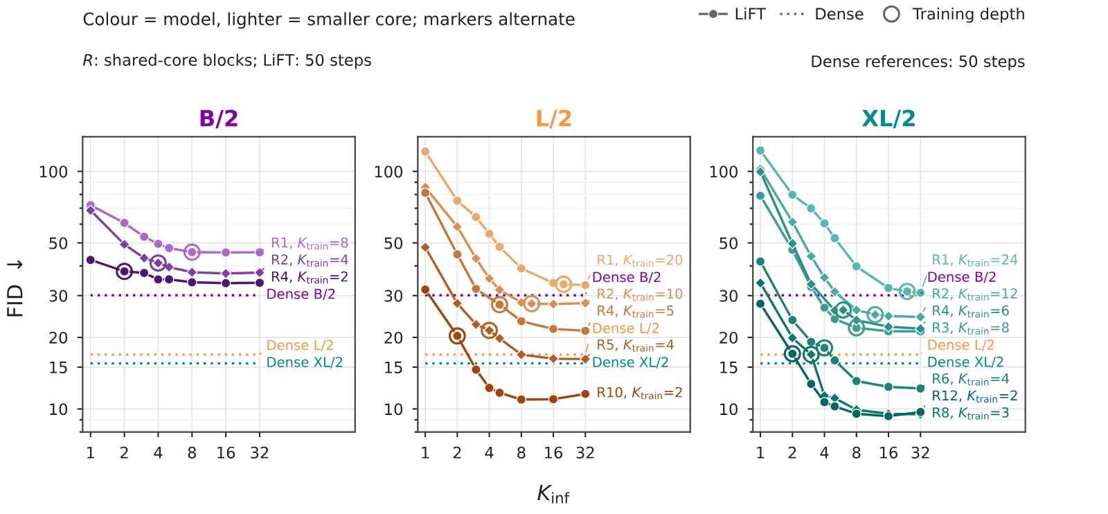
The gains are not uniform, and the paper is upfront about it:
- Large cores trained with few loops extrapolate best. XL/2 R12 goes 17.07 → 9.31 at 16 loops; XL/2 R8 goes 16.95 → 9.50 at 32; L/2 R10 goes 20.30 → 10.95 at 8.
- Single-block cores barely move: B/2 R1 goes 45.70 → 45.58. One shared block doesn't have the capacity, which matches the ELT result the paper cites.
- The curves turn up at 32. L/2 R10 rises from 10.95 to 11.57, XL/2 R12 from 9.31 to 9.71. Extrapolation works, but it has a sweet spot, around 8 to 16 loops for the best cores.
Checking "52% fewer inference FLOPs"
The headline in the abstract and the thread: LiFT-L/2 beats the dense DiT-XL/2 baseline by 3.34 FID with about 60% fewer parameters, 32% fewer training FLOPs and 52% fewer inference FLOPs. I checked every ratio against Tables 3 and 15. The settings are LiFT L/2 R10 at 50 steps and 8 loops (FID 10.95, 28.24 TFLOPs per image, 270.24M parameters, 61.98 EFLOPs to train) against dense XL/2 at 250 steps (FID 14.30, 59.31 TFLOPs, 674.82M, 91.10 EFLOPs). Then 1 − 270.24/674.82 is 60%, 1 − 28.241/59.308 is 52%, and 1 − 61.984/91.098 is 32%. All three are correct.
What the headline leaves out is the operating point it picked. Dense XL/2 at 250 steps is on its plateau. The same model at 100 steps gets 14.69 for 23.72 TFLOPs, and at that point LiFT's 28.24 TFLOPs is about 19% more compute, not 52% less. LiFT still wins on quality by a wide margin (10.95 against 14.69), with 60% fewer parameters and 32% less training. So the quality and parameter claims stand. The 52% comes from comparing against a dense model spending most of its compute on steps that no longer help, which is the paper's own point about steps saturating, used to make the saving look bigger.
The comparisons I'd lead with are less dramatic and fairer:
- Same scale, same training FLOPs: LiFT L/2 R10 at 25 steps and 4 loops gets FID 13.16 at 7.397 TFLOPs. Dense L/2 at 50 steps gets 16.94 at 8.069 TFLOPs. About 8% less compute, 41% fewer parameters and 3.8 FID better, from a checkpoint trained with the same budget.
- Against the bigger dense model at its default, the same LiFT setting against dense XL/2 at 50 steps (15.54, 11.862 TFLOPs) uses about 38% less inference compute, with 32% less training compute and 60% fewer parameters.
- XL/2 against XL/2: LiFT XL/2 R8 at 4 loops gets 11.36 at 15.25 TFLOPs; dense XL/2 needs 23.72 TFLOPs and 100 steps to reach 14.69.
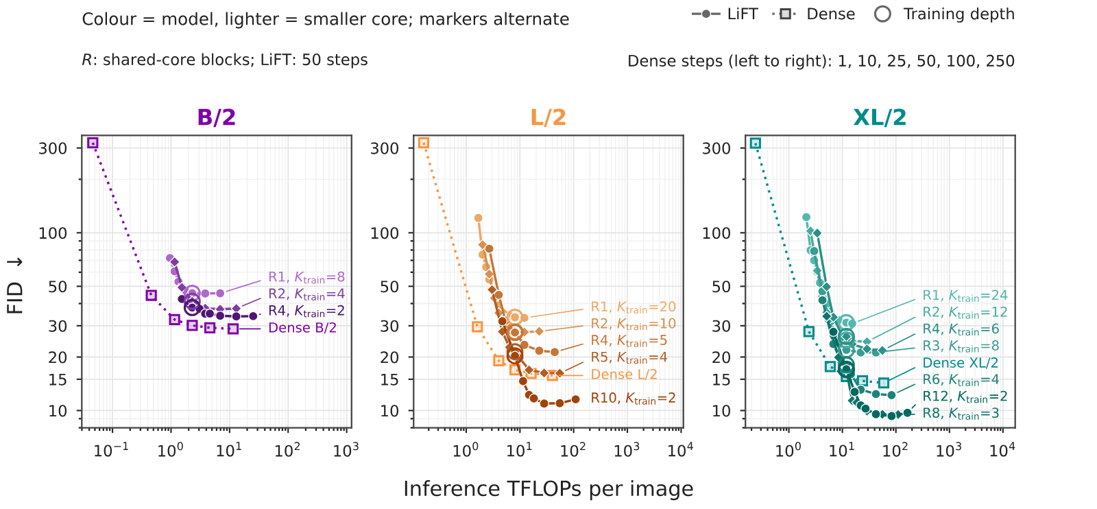
There are two more things the headline doesn't show. At its training depth, every LiFT checkpoint is worse than the same-scale dense model at the same cost: L/2 R10 scores 20.30 at two loops, dense L/2 scores 16.94. The paper explains this with an iso-depth result from looped language models, where a shared block is worth about half a unique one. The win only appears once you spend extra inference compute on loops. And at B/2 it never appears. The best LiFT B/2 result, 33.87, doesn't reach the 32.50 that dense B/2 gets at 25 steps. The authors' explanation is that the B/2 cores, at most 89M parameters, are too small for 32.8B training tokens. Plausible, and untested.
How to split a budget between steps and loops
So loops beat steps sometimes. When? The paper sweeps L/2 R10 over and , 24 settings at 50,000 samples each. That grid is the most useful thing in the paper if you would actually deploy one of these.
| T \ K | 1 | 2 | 4 | 8 | 16 | 32 |
|---|---|---|---|---|---|---|
| 10 | 48.6 0.94 TF | 33.6 1.61 TF | 19.0 2.96 TF | 15.3 5.65 TF | 15.1 11 TF | 16.4 22 TF |
| 25 | 34.8 2.35 TF | 22.6 4.04 TF | 13.2 7.40 TF | 11.4 14 TF | 11.4 28 TF | 12.1 54 TF |
| 50 | 31.8 4.71 TF | 20.3 8.07 TF | 12.3 15 TF | 11.0 28 TF | 11.0 55 TF | 11.6 109 TF |
| 100 | 30.6 9.41 TF | 19.4 16 TF | 12.0 30 TF | 11.0 56 TF | 11.0 110 TF | 11.5 218 TF |
Faded cells cost more than the budget. All settings use Euler sampling with no classifier-free guidance; dense L/2 trains with the same FLOPs as this checkpoint, dense XL/2 with about 47% more. Rows are integration steps T, columns are loops per step K.
Two rows of that table make the case for compute inside each step better than any prose. Hold loops at one and add steps: 48.61 at 10 steps, 30.59 at 100. Hold steps at ten and add loops: 48.61 at one loop, 15.29 at eight. The sampler can't fix a bad velocity estimate however many steps you give it. The loops fix the estimate.
It also cuts the other way. Sixteen loops at ten steps gets 15.09 for 11.027 TFLOPs, which is both worse and more expensive than four loops at 25 steps (13.16 at 7.397). Past a few loops, a ten-step Euler sampler is the bottleneck again, and the next unit of compute should go to steps. At the top end both axes flatten: eight loops gives 10.95 at 50 steps and 10.96 at 100.
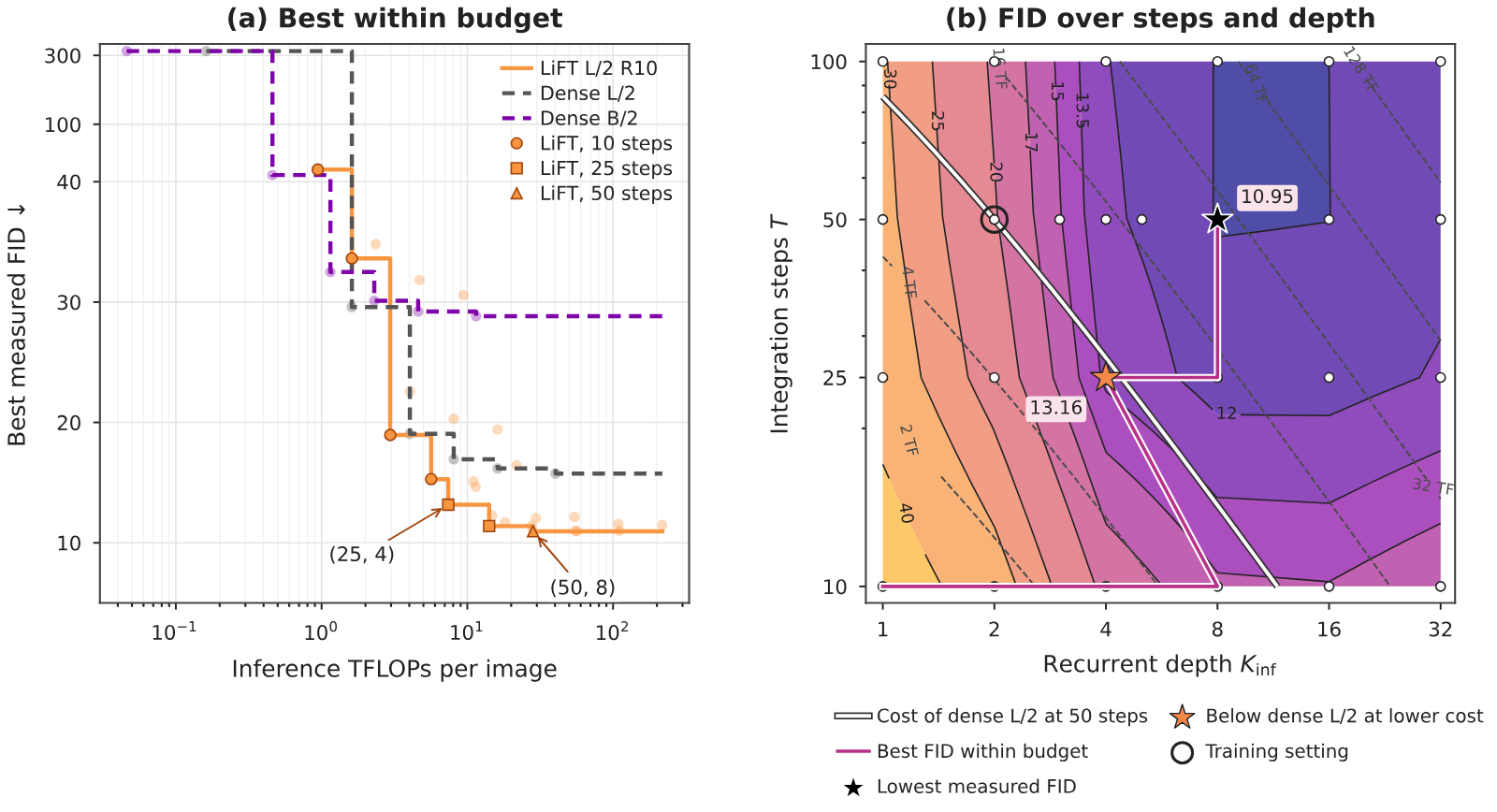
The pink path in panel (b) is the real recipe. As the budget grows it adds loops at ten steps, trades some of them for steps, adds loops again, and finally adds steps. If I were running this I'd pick a small set of (T, K) presets off that path and expose them as one quality knob. A single checkpoint covers the whole range, which is the property the authors care about most.
Velocity MSE barely moves; FID does
There's a number in Appendix B.4 that I think matters more than the paper suggests. Take L/2 R10, feed the same noisy inputs through grids of different depth, and measure the MSE of the final velocity against . For every grid with it sits between 0.7667 and 0.7689. FID over the same range of depths goes from 20.30 to 10.95.
No contradiction: it's the term from the decomposition above. At , most of the per-sample error against is the conditional variance of given , noise no network can remove, and it swamps the part the loops improve. The practical consequence: if you train something like this, validation velocity MSE will tell you almost nothing about whether more loops help. You have to sample. The paper does, with 50,000 images per setting.
What the pictures show, and what they don't
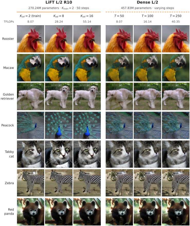
Look at the retriever and peacock rows. At its training depth LiFT produces the same kind of mangled animal the dense model does. At eight loops it is a dog, while more steps barely change the dense columns. The paper's whole argument fits in those two rows. But the caption says selected, so read it as an illustration and take the 50,000-sample FIDs as the evidence.
I tried to make my own strip through the demo with a different class, same seed, 1 to 16 loops. The first call came back, and then the Space's ZeroGPU quota for anonymous callers ran out for the day. So I have nothing to add here beyond the authors' images. The demo exposes class, seed, integration steps and (1 to 32) for the L/2 R10 checkpoint, plus dense L/2 and XL/2 at up to 250 steps. Its footer says "500k-step EMA checkpoints · SD-VAE · Euler sampling · no CFG", which matches the paper's protocol.
Where it sits among the other looped DiTs
Three neighbours make LiFT's choice clearer.
- Looped-DiT (SenseTime, covered earlier today) loops the middle of a text-to-image MMDiT and trains every intermediate loop toward the full output through a shared post-loop stack, which is deep supervision. It also found that loops beat steps at a matched per-image budget, which is LiFT's Q3 result from an independent group on a different task. LiFT doesn't cite it; the two appeared within weeks of each other.
- ELT adds self-distillation from a detached full-depth prediction to its intermediate exits. The paper cites it as the source of both negative results above, FID getting worse past training depth on ImageNet and quality peaking at 1.5 times training depth on video.
- LoopDiT (Chai) has the same prelude-core-output layout and depth conditioning, but trains with MeanFlow and keeps a prefix of its training schedule for shorter runs. LiFT re-spaces the full interval so every budget ends at . The paper reports LoopDiT found no advantage over a dense model at equal compute.
So the architecture isn't new. Prelude, shared core, depth embedding and input reinjection are all borrowed, and the paper says so. What's new is giving each loop a different target, a continuous coordinate for it, and the observation that this reuses flow matching's own construction. The authors call it "only light changes to the standard architecture", which is accurate.
What I'd want before using it
The results are on class-conditional ImageNet 256×256 with no classifier-free guidance. Guidance changes the velocity field a lot, and whether the depth curve survives it is the first open question. The authors list it as a limitation. The absolute FIDs are unguided numbers from a 500,000-update budget. They are fine for comparing these models with each other and say nothing about state of the art.
Every number comes from one training run and one sample set. The FID gaps that matter here are several points, much larger than seed noise usually is, so I'm not worried about the main claims. I would be worried about the 0.04-point differences between neighbouring settings.
Costs are analytic FLOPs. There is no latency, memory or energy measurement, and the paper says so. For this architecture FLOPs should track wall clock better than usual: every loop is a full-width block with no KV cache to carry, so a loop costs what a block costs. But the edge-device pitch in the conclusion needs a device to back it.
And the code isn't out. The tweet promises "the codebase, W&B artifacts, and checkpoints"; the paper's links say "Coming Soon". The method is simple enough that Algorithm 1 is close to a spec. Here it is in PyTorch, transcribed from the paper's pseudocode (Algorithm 1, lines 1 to 14). The prelude, core, head and embedding modules are placeholders:
# One LiFT training step, transcribed from Algorithm 1 of arXiv 2610.05538.
def lift_loss(x1, y, K, lam=0.01):
    B = x1.shape[0]
    x0 = torch.randn_like(x1)
    t = torch.rand(B, device=x1.device)
    xt = (1 - t.view(B, 1, 1, 1)) * x0 + t.view(B, 1, 1, 1) * x1
    u_star = x1 - x0

    # K-1 interior depths per example, sorted, then the endpoint s=1
    s = torch.sort(torch.rand(B, K - 1, device=x1.device), dim=1).values
    s = torch.cat([s, torch.ones(B, 1, device=x1.device)], dim=1)

    c = e_t(t) + e_y(y)
    h0 = prelude(xt, c)
    u0 = head(h0, c)
    b = u0.detach()                                   # anchor: stop-gradient
    loss = lam * F.mse_loss(u0, u_star)               # prelude loss, outside the average

    h = h0
    for k in range(K):
        sk = s[:, k]
        h = core(rms_norm(h) + h0, c + e_s(sk))       # reinject h0 every pass
        uk = head(h, c)
        target = (1 - sk.view(B, 1, 1, 1)) * b + sk.view(B, 1, 1, 1) * u_star
        loss = loss + F.mse_loss(uk, target) / K
    return loss
Sampling is the same loop with , no intermediate readouts and one Euler update per step. The paper also nudges the sorted draws apart by in FP64 so no two coincide; I left that out.
Would I use it? For a deployment where weights are the constraint and you want one checkpoint covering several quality and latency budgets, yes. 270M parameters doing better than a 675M model is a real saving in memory. For a server that only ever runs one budget, the case is weaker. A dense model at its best step count is a known quantity, and LiFT's advantage there is the cleaner 8 to 38% compute figures above, not 52%.
The idea I expect to outlast this paper is the target. "Give each loop a fraction of the correction, indexed continuously" doesn't depend on images or on flow matching's endpoint. Any looped model with a prediction at every pass, language models included, could try the same thing. The open question is whether there is an anchor as natural as when the output is a distribution over tokens.
How I checked
I read the arXiv HTML of 2610.05538v1 in full, including the appendices, and took every number in this piece from its tables (3, 4, 5, 6, 8, 9, 10, 11, 12, 15, 17) or its text. The X threads by both first authors were read through the fxtwitter mirror; they add the demo link and nothing that contradicts the paper.
I re-derived the FLOP accounting from the paper's Eq. 32, with tokens and . For L/2 () that gives 6.7235 GFLOPs per block per image. Dense L/2 at 50 steps comes out at 8.068 TFLOPs against the table's 8.069. LiFT L/2 R10 at 8 loops ( blocks) comes out at 28.239 against 28.241. Dense XL/2 at 250 steps comes out at 59.30 against 59.308. Training compute gives 61.96 EFLOPs for dense L/2 against 61.973. The small differences are the heads and embeddings I left out. The headline ratios (60%, 52%, 32%) and my alternative comparisons are plain divisions of table entries. One rounding note: 14.30 − 10.952 is 3.348, which rounds to 3.35, not the paper's 3.34. That only matters if the dense value printed as 14.30 is slightly below it, and either way it's the same result.
The figures are the paper's own: Figure 2 and Figures 3 to 5 were SVGs, which I rasterised at 1600 px on white; Figure 7 is the paper's PNG. The two widgets use the paper's equations and Tables 3 and 6 directly, with no interpolation. I read the demo's Gradio config to see what it exposes, and one call succeeded before the anonymous GPU quota ran out. I couldn't check anything that depends on code, since none is released.