Generative Trajectory Planning: a diffusion prior that proposes plans and learns from the ones search finds
mdjsonmcp2026-10-24 · 19 min · reinforcement-learning · diffusion · robotics · world-models
A 2:01 narrated explainer, drawn in code. Every number and picture in it is this article's own; the sources are below.
› transcript
Hi, I'm Sheave! This agent has no policy. It has a model that proposes whole plans, and it learns from the plans its own search finds. Sample whole action sequences from a diffusion model, improve them by search, then teach the model the winners. The state goes into a diffusion model over whole action sequences. It samples thirty-two plans. A beam search copies the best few and re-noises only their uncommitted actions, then denoises them. Five learned dynamics models roll each plan forward, and a reward model and value function score it. Repeat once per step of the horizon, then execute the first action and plan again. Learning reuses the same search. Plan from replayed states, scoring cautiously with the median model. The value function learns the planned returns. Noisy gradient steps push the winners uphill, against collapse. The diffusion model learns the elites, weighted by score. In the limit, each round does one thing. Take the current prior. Weight every plan by its exponentiated score. Good plans gain mass, and the expected score provably improves. A Gaussian has one mode, so two good routes around an obstacle average into a bad one. A diffusion prior keeps both routes. Pushing a block from pixels, the reinforcement learning baselines stay at zero. The Gaussian planner reaches thirty-three percent. This one, ninety-nine. And once trained, one sample from the prior is enough. Planning off, pick and place still succeeds ninety-nine percent of the time. Search is the teacher. Then the prior can act alone. The prior proposes, search improves, and the winners train the prior. Every source is in the full article. I'm Sheave. Bye!
Why read this
Notabletop 60%GTP's beam search and prior update from the equations and the JAX code, the tables re-read with their caveats, and released checkpoints run on CPU.
- Original analysis
- Runs on a consumer GPU
- A lasting reference
Robotics & embodiedNo licenceResearch paper
How this was scored
- Is it new?
- 2 of 3: A real new idea, method or capability
- Can I trust it?
- 2 of 3: Measures key facts from files, code or configs
- Can I run it?
- 2 of 3: Open code or weights with real limits
- Will I understand it?
- 2 of 3: Mechanism from first principles with figures
- Can I act on it?
- 2 of 3: A concrete recipe, numbers or comparison
- Will it last?
- 2 of 3: A reference for a year or more
- Does it affect many?
- 1 of 3: A specialist community
- Only here?
- 2 of 3: A teardown or measurement few others did
Score 67 of 100, ranked 189 of 607 rated articles. Each question is answered 0–3 by hand, and a 3 is rare. How articles are scored
Haldun Balim's thread opens with a question: "What if embodied agents could learn to plan instead of just learning how to act?" The method is Generative Trajectory Planning, GTP. In online reinforcement learning it does away with the policy. A diffusion model proposes whole action sequences, a search refines them, and the sequences the search finds become the diffusion model's next training data. Planning teaches the planner.
The paper is arXiv 2610.18677, by Balim, Yilun Du and Na Li at Harvard, accepted at NeurIPS 2026. The JAX code is at haldunbalim/GTPlanning, and the trained models, one per environment with a checkpoint every 100k steps, are on Hugging Face. I read all three. I also ran a released checkpoint on a CPU, with and without planning, and I built a small toy you can play with below. The numbers mostly hold, with two table footnotes, and the price is paid in training compute, not when acting.
- branch
- HEAD
- tests
- none found
- source
- 236.0 kB
- commit date
- 2026-10-15
by size of tracked source at this commit, file counts in brackets; docs, data and vendored trees excluded
local clone, 2026-10-24 at ec5ff66 — branch, commit, commitDate, fileCount, hasTests, languages
Two camps, and the gap between them
RL compresses the future into a value function and learns a one-step policy against it. Acting is one forward pass. But the value function bootstraps one step at a time, so reward information travels backwards slowly, and exploration is noise on individual actions, which rarely produces a coherent behaviour like "go round the block, then push".
Trajectory optimization, or model predictive control (MPC), plans explicitly. At every step it solves
over an action sequence of horizon , executes only the first action, and solves again next step. is an optional terminal value for everything past the horizon. Sampling solvers such as CEM and MPPI draw candidate sequences from a Gaussian, score them, and refit the Gaussian to the best. The cost is a fresh high-dimensional optimization at every step. The quality is capped by the proposal: a Gaussian has one mode, and good action sequences often come in several.
GTP keeps the MPC loop and swaps the Gaussian for a learned generative model. Instead of optimizing from scratch, it samples from a distribution that has already learned where good plans live.
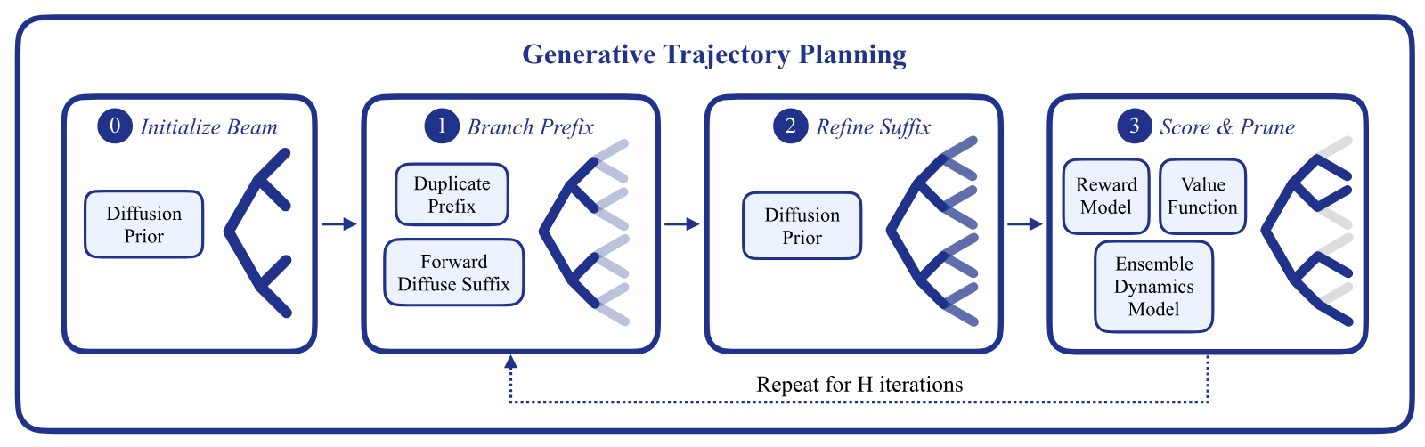
Four learned parts
All four networks learn online from the agent's own replay buffer.
- A diffusion prior over -step action sequences, conditioned on the current state. In the code it is a temporal U-Net with FiLM conditioning and denoising steps, trained with the standard noise-prediction loss.
- A dynamics ensemble of MLPs, each predicting the change in state, each trained on its own bootstrap resample of the minibatch so they disagree where data is thin.
- A reward model with a second head that predicts termination. Rollouts multiply rewards by a running survival probability, so a plan that falls over stops collecting reward.
- A value function that bootstraps everything past the horizon.
Locomotion runs at , manipulation at (paper Table 3, and the released configs agree).
How it plans at test time
Score a candidate prefix of length by rolling it through ensemble member :
then collapse the five estimates with a rule . The rule is where exploration lives. When the agent acts during training it uses max: a plan is attractive if any one model thinks it pays off, which is optimism under uncertainty. When it builds learning targets it uses median, so one over-optimistic model cannot leak into the value function.
The search is Algorithm 1, a beam search with a diffusion twist:
- Initialize. Sample sequences from the prior and keep the top under , the one-step score.
- Branch. Copy each surviving sequence times.
- Refine. Forward-diffuse each copy for noise steps, then denoise it back with the prior, restoring the committed prefix after every denoising step. Only the uncommitted suffix changes.
- Prune. Keep the top under , which scores one more committed action.
Repeat steps 2 to 4 for and return the best full sequence. Execute its first action. Several beams run in parallel so the search can hold more than one mode of the prior. The thread's reply to "doesn't re-noising every step blow up latency?" is that only a few re-noising steps are used. That checks out: against for a fresh sample.
The budget is small. Paper Table 3 lists 32 total samples, 4 beams, beam width and branching factor , so candidates at every depth. The code spells it differently: beam_k: 8 is the total kept across all beams, num_beam: 4, and beam_d = num_samples // beam_k = 4. Same numbers. At that is sequential denoiser passes per decision (reasoned, from the config). The released Fetch checkpoints differ in one setting the paper never mentions: their configs say chunk_size: 2, so the search commits two actions per depth, four depths instead of eight, and passes (measured from the Hugging Face configs; the arithmetic is reasoned). The repo's own gtp-manip.yaml uses 1, as Algorithm 1 describes. The JAX implementation also avoids re-rolling the committed prefix: it caches the predicted states, rewards and survival terms of the prefix and runs the dynamics only for the newly committed step at each depth (measured, from gtp/algo/gtp.py). Because refinement never touches the prefix, the cache stays valid.
One more code detail: get_eval_action plans with up_agg, the cautious rule, not the optimistic max used while collecting data (measured). The policy in a results table is not quite the one that explored.
How it learns to plan better
"Learns to plan better through experience" is two regression targets built from the planner's own output.
The value function is trained on planned returns, not on one-step TD targets. For a state in the batch, run the planner, take its best sequence , and read off every prefix return for . Short prefixes lean on the current value estimate; long ones lean on the dynamics model. GTP mixes them with weights from cross-ensemble disagreement:
where is the variance of across the five models. This is STEVE's inverse-variance weighting with a softmax on top. It is how long-horizon reward information gets into in one update instead of .
The prior is trained on the plans. Run the beam search, add Langevin perturbations of the winners, keep the top as elites, and weight them by their scores:
The exponential weighting is MPPI's. The difference is where it lands: MPPI uses it to refit a Gaussian for one state and throws it away, while GTP distills it into one network that serves every state. That is the amortization the abstract talks about. The temperature is not hand-tuned: it is adapted so that the effective sample size of the four elite weights stays at a target of 0.8. As the prior sharpens and the elites' scores bunch together, a fixed would flatten the weights to uniform.
Two details stop the loop from eating itself. A prior trained only on its own best samples collapses: the elites look like what it already produces, and learning stalls. So four Langevin steps push the elites uphill on with noise, , injecting candidates the prior would not have proposed. And the planning horizon grows linearly from 1 to over the first 300,000 environment steps (350,000 for manipulation), so the models learn short predictions before they are trusted with long ones.
The theory section idealizes the prior update as with the models held fixed, and proves (Theorem 3.1) that each step gains at least in expected score and that the prior concentrates on near-optimal sequences, provided the starting prior gives them some probability. That proviso is exactly what the Langevin step is for.
The loop on a toy you can enumerate
The widget below is ours, not the paper's. It applies the idealized update exactly to every possible plan in a grid world small enough to list: a 7 by 5 grid, a three-cell wall in the middle column, start on the left, goal on the right. A plan is six moves from right, up, down and left, so there are plans and the prior is a table of 4,096 probabilities. Reward is per move off the goal, and the value function is the true shortest-path distance, so the best possible score is . Twelve plans reach it, six over the wall and six under it (measured, by enumeration). The planner is Algorithm 1 with the paper's budget of 4 beams, width 2 and branching factor 4. "Re-noise and denoise the suffix" is replaced by its exact limit: resample the uncommitted moves from the prior, conditioned on the committed ones.
Three things show up (all measured on the toy). From a uniform prior, a plan drawn at random scores on average and only 0.29% of the mass sits on the best plans. Best-of-32 sampling, the paper's "No plan." ablation, finds a plan in 7.5% of 200 seeded calls, while beam search with the same 32 candidates per depth finds one in 97.5%. That gap is flattered by the toy's perfect value function, which makes even the one-step score a reliable guide. Second, each update gains at least times the KL divergence, as the theorem says: at , the first update gains 1.58 against a bound of 0.83. After four updates 89.4% of the mass is on the twelve best plans. Third, look at the dashed line. It is the prior's average move sequence, which is where a single Gaussian fitted to the same plans would aim. Because the good plans split evenly above and below the wall, their average goes straight into it. That is the paper's argument against Gaussian proposals in one picture. With a uniform starting prior, updates at temperature equal one update at , so the slider and the buttons trade off (reasoned).
Where it sits
- Diffuser (Janner, Du, Tenenbaum, Levine, 2022) diffuses whole state-action trajectories offline and plans by guided sampling. Decision Diffuser (Ajay, Du and colleagues, 2023) conditions a state-trajectory diffusion model on return and recovers actions with inverse dynamics. Both learn from a fixed dataset, and in both the generative model is the planner. GTP is online, diffuses actions only, keeps dynamics in a separate ensemble, and treats the diffusion model as a proposal that something else scores. Yilun Du is an author on all three.
- MPC with CEM or MPPI is GTP with a Gaussian proposal refit from scratch every step. The paper's CEM-MPC and CEM-MPC-V baselines share GTP's own dynamics and value networks, so they isolate exactly that swap.
- DreamerV3 trains an actor-critic inside a learned world model and acts without planning. GTP plans with its models and has no actor.
- TD-MPC2 is the closest relative: a learned latent model plus MPPI planning, with a Gaussian policy prior and one-step TD value learning. GTP replaces the Gaussian with a diffusion prior over sequences, the one-step targets with multi-horizon planned returns, and the single model with an ensemble.
- Diffusion-policy RL (DPMD, QSM) trains a diffusion model as a one-step policy. GTP's prior loss is DPMD's reweighted denoising loss, applied to planner-scored sequences instead of Q-scored actions.
On this site, H-JEPA plans by gradient descent on actions through a learned latent world model, and its levels split the horizon instead of searching it. Flex-π denoises actions and futures together in one robot model. Adapt-1 Machina drops the critic because its simulator grades every attempt, which is the extreme opposite of GTP's fully learned evaluator.
The benchmarks, checked against the tables
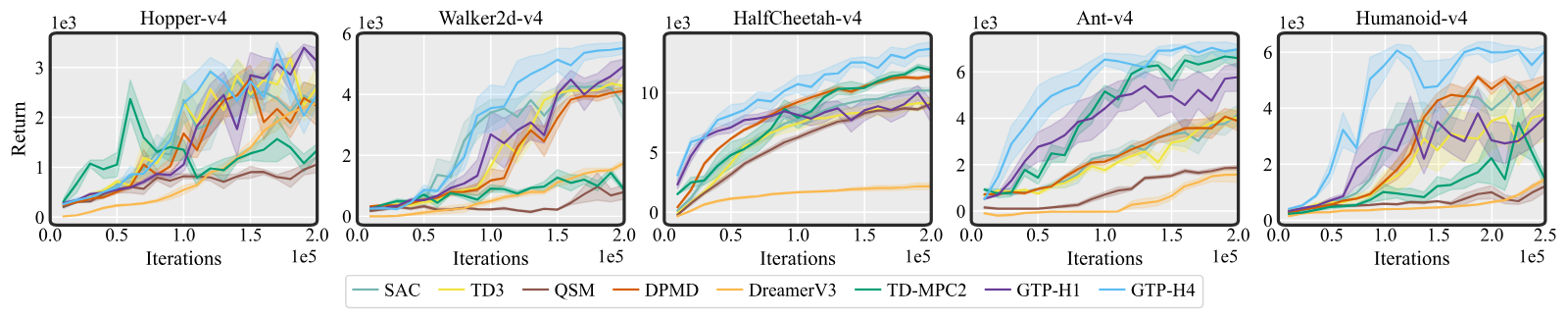
Locomotion. Five MuJoCo tasks, 1M environment steps, 5 seeds (reported, Table 1).
| Task | best baseline | GTP-H1 | GTP-H4 |
|---|---|---|---|
| Hopper-v4 | SAC 3351 ± 39 | 3398 ± 71 | 3525 ± 49 |
| Walker2d-v4 | SAC 4453 ± 158 | 5007 ± 212 | 5546 ± 201 |
| HalfCheetah-v4 | TD-MPC2 12216 ± 267 | 10372 ± 439 | 13944 ± 498 |
| Ant-v4 | TD-MPC2 7339 ± 119 | 6207 ± 418 | 7369 ± 73 |
| Humanoid-v4 | DPMD 5269 ± 44 | 4596 ± 785 | 6660 ± 132 |
The thread's "highest return on all 5 tasks" is true of the means. On Ant the lead is 30 points with standard errors of 73 and 119, which is a tie (reasoned). Two footnotes matter more.
First, the numbers are each run's best evaluation, not its final one. Table 1's caption says "mean returns", but the ablation figure, whose full-GTP entry is 5546 ± 201, and the beam-size table, whose default entry is 13944 ± 498, both call the same figures "best mean returns" (reported, Figure 5 and Table 4). The training curves agree: GTP-H4 on Hopper peaks around 3,400 and ends visibly lower (read by eye from Figure 3). Best-checkpoint reporting flatters every method, and only the CEM baselines are documented ("the best result over the last three checkpoints").
Second, Ant is not run with the default rule. With max for acting and median for targets, the termination-heavy Ant degraded, so it uses min for targets and median for acting (reported, Appendix D, Figure 8). That is a per-environment choice made after seeing a failure, and it is disclosed.
The released checkpoints are not the table's runs either. The model card lists HalfCheetah at 14885 ± 192 and Ant at 7138 ± 60 at 1M steps (reported), single models rather than five-seed means.
Manipulation. Success rates after 1M steps, 5 seeds, 100 trials each, (reported, Table 2).
| Task | SAC / TD3 / DPMD | DreamerV3 | TD-MPC2 | CEM-MPC-V | GTP |
|---|---|---|---|---|---|
| FetchPush | 6 / 6 / 6 | 7 | 67 ± 17 | 78 ± 6 | 100 ± 0 |
| FetchPick&Place | 3 / 3 / 3 | 1 | 99 ± 0 | 68 ± 5 | 98 ± 1 |
| FetchSlide | 1 / 5 / 5 | 0 | 70 ± 3 | 67 ± 1 | 76 ± 3 |
| PushT-Vision | 0 / 0 / 0 | 0 | 0 ± 0 | 33 ± 4 | 99 ± 1 |
The thread's "every learning baseline is at 0%" on PushT from pixels holds for SAC, TD3, QSM, DPMD, DreamerV3 and TD-MPC2. The two CEM planners are not at zero, but they reuse GTP's own learned models. On FetchPick&Place TD-MPC2 finishes a point higher than GTP; the paper's claim there is speed, and Figure 4 shows it. On FetchPush the TD-MPC2 average hides that it failed to converge in 2 of 5 seeds.
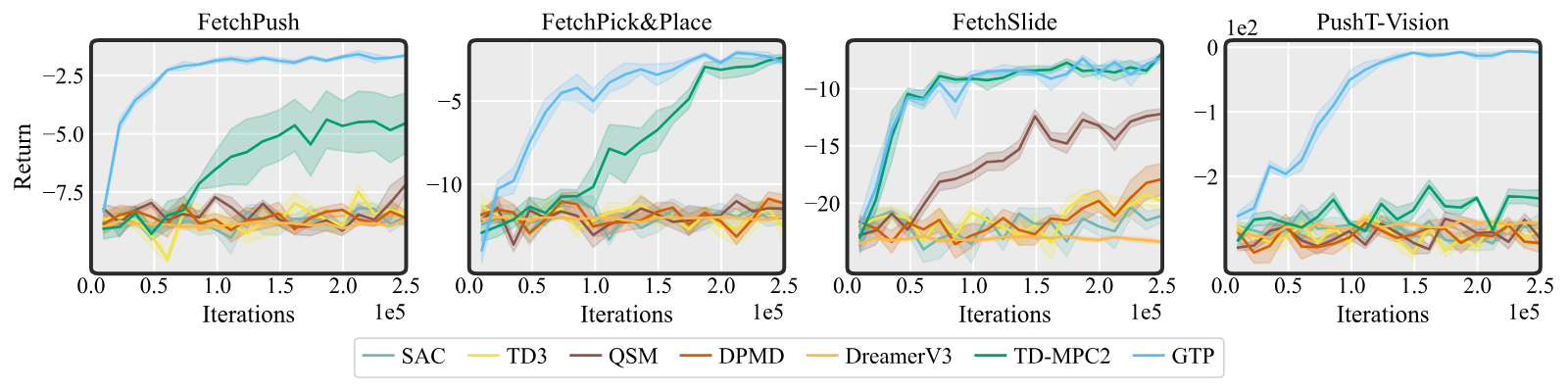
The PushT gap is speed, not a ceiling. With 3M steps instead of 1M, TD-MPC2 reaches 97 ± 1 against GTP's 99 ± 1, while SAC, TD3, QSM, DPMD and DreamerV3 stay at 0 (reported, Table 5).
What matters inside GTP (best mean return, reported, Figure 5; the figure does not name the task, but its full-GTP entry is Table 1's Walker2d number): dropping Langevin augmentation falls to 1652, a single dynamics model instead of five falls to 1998, best-of-32 filtering instead of beam search falls to 3177, and one-step TD targets fall to 4556, all against 5546 for the full method. The ensemble and the anti-collapse step matter most.
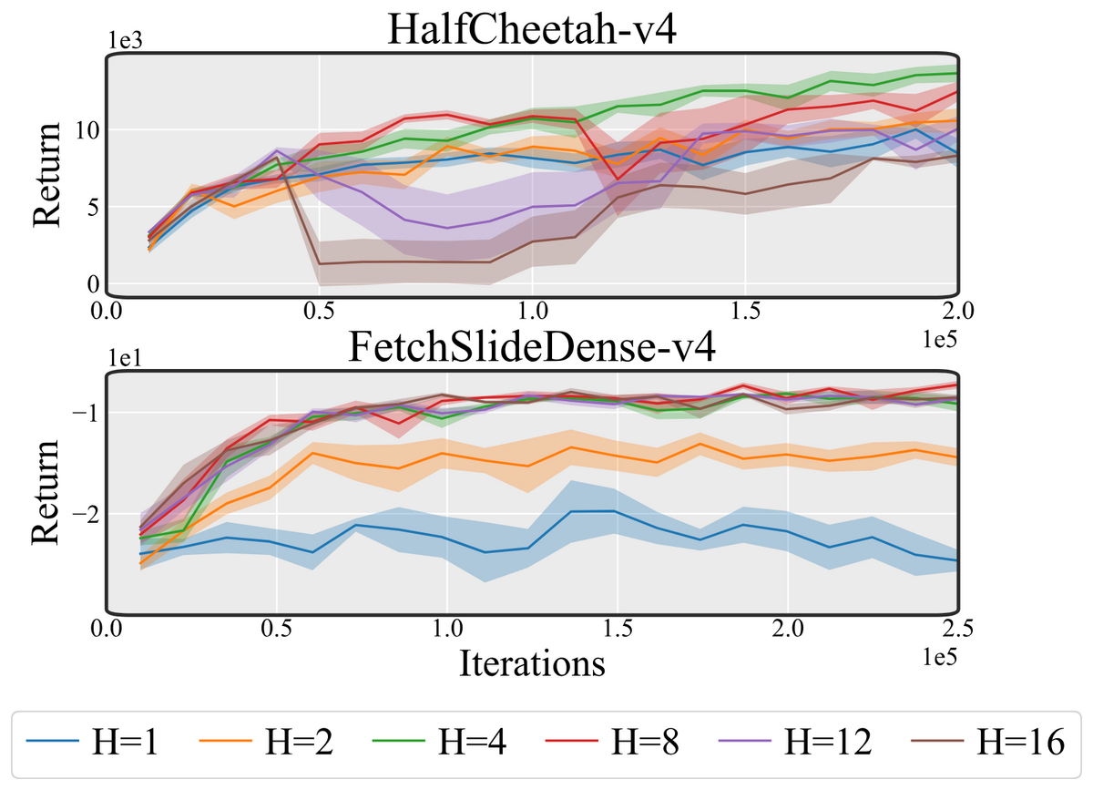
Horizon. On FetchSlide, barely improves while every horizon from 4 to 16 trains to a similar high return, which is the thread's claim. On HalfCheetah, past returns go down, and collapses for a long stretch mid-training. The paper attributes that to dynamics error in contact-rich locomotion. Longer horizons are not free; they are as good as the model.
What it costs
On one RTX 5090, GTP at picks an action in 34.25 ms against 36.20 ms for TD-MPC2 at the same horizon (reported, Table 6). Acting is not the problem. Training is: an update takes 157.15 ms against 3.99 ms, because every update runs a beam search for every state in the batch. That is about 39 times TD-MPC2 per update (reasoned). Caching each transition's elites and refreshing them every 10 updates brings it to 19.12 ms, 8.2 times cheaper, with FetchSlide dropping from 76 to 69 and the other three tasks within two points (reported, Appendix J).
The more interesting result is in Appendix K. On FetchPick&Place the paper samples a single sequence from the prior, with no beam search and no scoring, and gets 99% success at 8.61 ms an action, against 98% at 34.25 ms with the full 32-sample planner (reported, Table 7). Once trained, the prior is the policy. The author makes the same point in a reply: "once the policy is trained, planning is not necessary anymore". Executing 8 actions between replans still gets 92% (reported, Table 8).
What I ran
The repository ships scripts/eval.py, which pulls a config and a checkpoint from Hugging Face and rolls out episodes. I ran it on a shared 4-core cloud VM, CPU only, pinned to 2 cores at the lowest priority, with JAX 0.6.0 as the repo pins it. I installed only what the evaluation imports and stubbed the logging packages (wandb, tensorboardX, orbax, matplotlib) that it never calls. My wrapper calls the repo's own build_algo, load_state and evaluate unchanged. For the planning-free run it sets one sample and a horizon of 1, which makes the code return the prior's single sample without a beam search. The checkpoint is FetchPickAndPlaceDense-v4 at 1M steps, planning horizon 8, chunk size 2.
| Setting | Episodes | Success | Mean return | ms per action, CPU |
|---|---|---|---|---|
| Released planner, 32 samples, beam search | 10 | 10 of 10 | −2.23 | 1023 to 2463 |
| Planning-free, 1 sample from the prior | 20 | 20 of 20 | −2.27 | 40.3 to 46.3 |
All measured. Per-action time is the median of 30 single-observation calls after JIT compilation, and the range is two runs: one under lighter load, one with the load average near 14 while other jobs shared the machine. On this machine the planner is 25 to 53 times slower than a single prior sample (reasoned, 1023 over 40.3 and 2463 over 46.3), against 4.0 times on the paper's GPU, where the 32 candidates run in parallel and the sequential depth dominates. Success and return are the same with and without planning, and the planning-free result matches Table 7: the released prior solves the task on its own. My sample is small, and Fetch episodes are only 50 steps, so read it as "consistent with the paper", not as a second measurement of 99%.
What I did not run: training. One update at is 157 ms on a 5090; a 1M-step run on two CPU cores is out of reach. Everything about learning curves, ablations and baselines above is the paper's.
Where it breaks
- Training compute. About 5 times TD-MPC2 per update even with elite reuse (reasoned, 19.12 over 3.99 ms). It pays in GPU hours to save environment steps.
- Long horizons need good models. Planning trusts the ensemble, and the ensemble's errors compound.
- Aggregation is a tuning knob. Optimistic max failed on Ant, where termination punishes plans that only one model believes.
- No licence file. The repository has no
LICENSE;setup.pysays "BSD" next to an "Anon Author" placeholder. Until that is fixed, the code is not clearly reusable. - Simulation only. Gym MuJoCo, Fetch and a 2D PushT. No hardware.
The thread's last post argues that generative models in online RL are "best used as proposal distributions for planning". The evidence supports a narrower version: a proposal distribution trained on its own search results ends up good enough to act alone. Planning is the training signal more than the runtime.