2026-10-13 · 27 min · diffusion · flow-matching · distillation · image-generation · diffusion-transformers
Why read this
Notabletop 60%Flow-renoise, flow-map and data-space rollouts derived side by side, the paper's tables rechecked, and its Algorithm 1 rerun on a 2D toy.
- Original analysis
- A lasting reference
- A new technique
Image & video generationNeeds datacenter GPUsResearch paper
How this was scored
- Is it new?
- 2 of 3: A real new idea, method or capability
- Can I trust it?
- 2 of 3: Measures key facts from files, code or configs
- Can I run it?
- 1 of 3: API-only, gated or restrictive licence
- Will I understand it?
- 2 of 3: Mechanism from first principles with figures
- Can I act on it?
- 2 of 3: A concrete recipe, numbers or comparison
- Will it last?
- 2 of 3: A reference for a year or more
- Does it affect many?
- 1 of 3: A specialist community
- Only here?
- 2 of 3: A teardown or measurement few others did
Score 62 of 100, ranked 248 of 513 rated articles. Each question is answered 0–3 by hand, and a 3 is rare. How articles are scored
When I took FastH3 apart a few weeks ago, one line in its checkpoint metadata stuck with me: dmd_denoising_steps: [999, 749, 500, 250]. Four network calls, at four fixed noise levels, for every video, every prompt, every pixel. As far as I could tell nothing about it was specific to that model. It is the uniform trailing schedule that few-step work on diffusion transformers treats as the default, and in the FastH3 write-up it was simply there, baked into a 33B student.
So when Shanchuan Lin (Peter Lin on X) posted Few-Step Generation via Data-Space Iteration, with a thread that opened on exactly that complaint, I read it the same day. Lin is the person behind SDXL-Lightning, AnimateDiff-Lightning and the adversarial post-training work at ByteDance Seed, so few-step distillation is his day job. His claim is that the schedule is not a hyperparameter to tune better. It should not exist.
What surprised me is how small the change is. The paper's own code puts the new rollout next to the old one, and the difference is about five lines. The training loss is untouched. Everything interesting is in what gets passed from one network call to the next.
What a flow model actually gives you
Start from the model being distilled. A flow-matching model is trained on straight lines between a data sample and Gaussian noise . The paper uses the convention where is clean and is pure noise:
The network learns the velocity , whose per-pair target is . To sample, you draw noise and integrate the ODE from back to . The teacher here is the public SiT-XL/2 checkpoint, and the paper's Table 3 shows the price of doing that properly: FID 8.26 at 250 network calls without guidance, 2.06 with guidance, which doubles the calls to 250×2.
One identity carries most of what follows. If you know the velocity at , you can jump straight to a guess at the clean endpoint:
This is -prediction. It is exact for the straight line of a single pair, and for the learned average velocity it gives the average of all clean images consistent with . At high noise that average is blurry, because many different images are consistent with almost pure noise. Pixel-space models such as JiT go further and make the network output directly, for a different reason (noise is high-dimensional and the data manifold is not), which I covered in the PixelUMM piece. Keep the identity in mind. Data-space iteration turns out to be this formula evaluated at , forever.
Two ways to spend four calls
Distillation trades the 250-call integral for a generator that gets there in a handful. The paper sorts existing few-step generators into two families, and the split is about what state crosses the gap between calls.
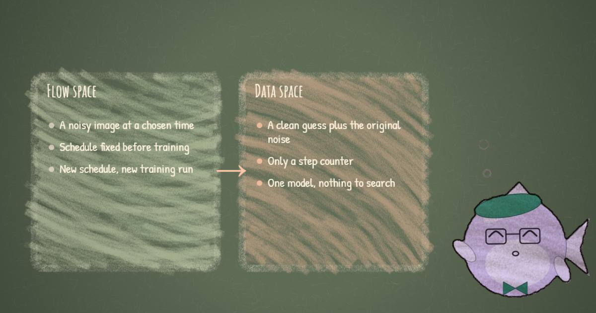
The first family, which the paper calls flow-renoise, passes a noisy image at a chosen time. At schedule point the generator predicts a clean image, and the sampler mixes that prediction with fresh noise to land at the next point:
Multistep consistency-model sampling works this way, and so does the original DMD. Every intermediate output is a complete image, which is convenient: you can stop after any call.
The second family, flow-map methods, also passes a noisy image, but learns the jump itself. The generator takes to directly, with no fresh noise:
Progressive distillation, SDXL-Lightning, shortcut models and MeanFlow are in this family by the paper's sorting. MeanFlow learns an average velocity over an interval and steps ; Phased DMD, the baseline the paper uses here, trains each interval with a distribution-matching loss. The intermediate states are not images, they are noisy latents at time , so a four-step flow-map model only has a four-step answer.
Both families need a list . For a model you sample with an ODE solver, that list is an inference-time choice. For the generators that matter in production it is not, because they are trained by self-rollout: during training, the generator runs its own earlier steps to produce the inputs for the step being trained. Streaming video distillation such as Self Forcing, the recipe behind StreamRender-H3, works this way. The states the student sees during training are defined by the schedule, so a different schedule means a different training run. Lin's thread says this is where the idea came from: choosing a discretization was a practical problem while they were working on autoregressive streaming video with self-rollout distillation.
There is also a softer argument in the introduction. One global advances every sample, and every spatial location within it, through the same denoising schedule, and there is no reason a goldfish and an ostrich, or a sky and a face, want the same step sizes. I will come back to how much of that the paper actually tests.
The change: pass the clean guess
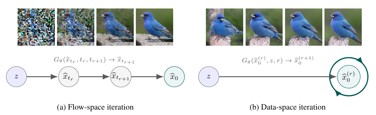
Data-space iteration keeps a clean-image estimate as the state. Start it at zero, then apply one shared generator times, handing it the current estimate, the original noise and the step index :
No fresh noise is added between calls, so nothing the model already got right is destroyed. No intermediate flow time is ever constructed, so there is no schedule to pick. Each call is trained to output the best finished sample it can, given what the previous call produced.
The implementation is where it gets neat. They build from the pretrained velocity network with three edits: the noise goes through the original input projection; the current estimate gets its own new projection, summed with the first; an embedding of is added to the timestep-conditioning path. The original time input is pinned at , and the output is
This is the -prediction identity from above with and . So every call is the teacher's one-jump-from-pure-noise prediction, with a side channel carrying the previous answer. Read the initialization with that in mind. The new projection has no bias (Appendix A), and the first estimate is all zeros, so on the very first call the new input contributes exactly nothing. At initialization, call one is the teacher's single-step -prediction from noise, plus the embedding drawn from . Training only has to teach the later calls how to use the side channel.
The appendix gives the parameter bill, and I redid it because "the model gets smaller" is a strange claim for a method that adds inputs. SiT-XL/2 has 675,129,632 parameters. The paper says the new projection and the embedding add 24,192, and dropping the timestep MLP in favour of a constant embedding removes 1,626,624, for 673,527,200. The total checks out: 675,129,632 + 24,192 − 1,626,624 = 673,527,200. The pieces mostly check out too. A bias-free 2×2 patch projection from a 4-channel latent into 1,152 dimensions is 16 × 1,152 = 18,432 weights, and the remaining 5,760 is exactly five 1,152-wide vectors, which fits an embedding table for the step index with one spare row. DiT's timestep MLP (256 → 1,152 → 1,152, with biases) is 1,624,320 by my count, 2,304 short of the paper's figure. That gap is two 1,152-wide vectors and I could not tell from the text what they are. The saving is real either way, and it comes from the fact that a model that never sees does not need the network that embeds it.
Training it with DMD, unchanged
The paper's second claim is that this is a drop-in change for distribution matching distillation. To see why, it helps to see what DMD optimises.
DMD wants the generator's output distribution to match the data distribution, and measures the mismatch with a reverse KL. The gradient of that KL with respect to a generated sample is the difference of two scores: the data's score and the generator's own score. Neither is available directly, so DMD estimates both at a blurred version of the sample. Take a generated , noise it to a random level , and ask two flow models for their velocity there:
- : the frozen teacher, which knows the data distribution at every noise level.
- : a copy of the teacher that is continually retrained on the generator's own noised samples, so it knows the generator's distribution.
Where the two disagree, the generator's samples are in the wrong place, and the difference points the way to move them. In the paper's velocity form:
The stop-gradient makes the bracket a fixed arrow, and the dot product with turns it into a gradient on the generator. The fake model is trained alongside with a plain flow-matching loss on the generator's noised samples, four fake updates per generator update here.
Nothing in that loss cares how was produced, and the drop-in claim rests on exactly this. Training picks a step , runs the first calls without gradients, runs call with gradients, and applies DMD to its output. The only addition for data-space is that is conditioned on , because each step has its own output distribution to track. The paper's Algorithm 1 prints the two rollouts side by side; this is the data-space one, verbatim:
# arXiv 2610.12102, Appendix E, Algorithm 1
def rollout_data_space(gen, z, c, r, track_grad):
    x_hat = torch.zeros_like(z)
    for i in range(r + 1):
        with torch.set_grad_enabled(track_grad and i == r):
            x_hat = z - gen(x_hat, z, c, i)
    return x_hat
and the flow-renoise one it replaces:
def rollout_flow_renoise(gen, z, c, r, track_grad, R=4):
    x_hat = torch.zeros_like(z)
    for i, t_r in enumerate(torch.arange(R, 0, -1, device=z.device)[:r + 1] / R):
        t_r = t_r.expand(z.shape[0])
        t_r4 = t_r[:, None, None, None]
        eps = z if i == 0 else torch.randn_like(z)
        x_tr = (1.0 - t_r4) * x_hat + t_r4 * eps
        with torch.set_grad_enabled(track_grad and i == r):
            x_hat = x_tr - t_r4 * gen(x_tr, t_r, c)
    return x_hat
Put them next to each other and the whole paper is visible. The renoise loop computes a time from the schedule (arange(R, 0, -1) / R is the uniform 1, 0.75, 0.5, 0.25), draws fresh noise after the first call, builds a noisy input, and converts the network's velocity to with . The data-space loop has no time, no fresh noise, and converts with . Same dmd_step afterwards. Since only one call per training step carries gradients either way, there is no extra memory or compute against a matched DMD baseline, which the paper states and the code makes obvious.
The setup is deliberately bare. No GAN loss, no extra regression term, which the paper says is so the iteration method is the only thing that varies. , Adam at , batch 256, 40 epochs, with , EMA 0.9999, TF32. The appendix says every model reproduces in about a day on one eight-GPU server with 80 GB cards.
Watching three rollouts on a toy
There is no released code beyond the two algorithms in the appendix, and a SiT-XL/2 DMD run is a day on eight 80 GB GPUs. So I did the next best thing and ran the paper's Algorithm 1 and 2 on a problem small enough to see: a ring of eight Gaussian blobs in 2D, where the teacher's velocity can be written down exactly.
The setup copies the paper wherever it can. Three small generators (three hidden layers of 64, SiLU) get the three rollouts from the appendix: data-space and flow-renoise from Algorithm 1, flow-map with Phased DMD's re-noising from Algorithm 2. All three train with the same DMD step, , , Adam with , cycling through 0 to 3, the uniform schedule, 6,000 generator updates and three seeds each. I made two shortcuts that only work in 2D. The "real" velocity is the mixture's exact probability-flow velocity, not a teacher network. The "fake" velocity is computed exactly from a fresh batch of 512 of the generator's own samples at the same step, rather than learned by a second network. Nothing here starts from a pretrained model, and nothing here is ImageNet.
Two things came out, and only one of them agrees with the paper.
The behaviour reproduces cleanly. I took 240 shared noise draws and asked which of the eight blobs each one lands in after the first call and after the fourth. Under flow-renoise, 198 of the 240 end up in a different blob from where call one put them. Under data-space, 14 do. Figure 2's goldfish-to-carrot effect survives the trip down to two dimensions: re-noising to throws away which mode you were in, and the next call picks again. The mean distance a point moves between calls tells the same story, about 1.86 then 0.89 then 0.30 for flow-renoise against 0.26, 0.12 and 0.07 for data-space, averaged over seeds. Follow one dot in the widget and you can watch it.
The ranking does not reproduce. I scored each method with a sliced Wasserstein distance against 20,000 draws from the ring, scaled by 100; two independent draws of the ring itself score 1.39. At four calls, averaged over the three seeds, flow-map scores 4.33, data-space 6.17 and flow-renoise 6.73. Data-space does improve with every call, 9.40 then 7.05, 6.39 and 6.17, while flow-renoise barely moves from 6.98, so the "every extra call buys something" shape is there. But in this toy the flow-map generator wins clearly, and data-space is the worst of the three after one call, which is the CIFAR-10 pattern rather than the ImageNet one.
I do not read that as evidence against the paper. A 2D ring has nothing like the per-sample and per-region variation the paper's argument relies on, my generators are tiny and start from scratch rather than from a teacher, and my exact "fake" is not the learned one. What the toy does show is that the mechanism is real and does not need ImageNet to appear: passing a clean guess instead of a re-noised one turns iteration from resampling into editing. Whether editing also wins on quality is the empirical question, and for that the paper's tables are the evidence, not my ring.
The numbers, and what they are measured against
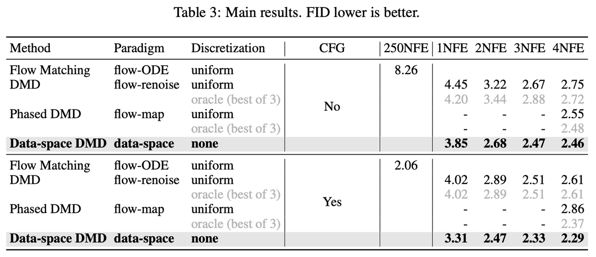
Read the table in two passes, as the paper does.
The first pass is the standard setting: everyone uses the uniform schedule [1.0, 0.75, 0.5, 0.25], which the paper notes is what prior few-step work on this architecture uses. Data-space wins every column. Without guidance it reaches 2.46 at four calls against 2.75 for DMD and 2.55 for Phased DMD; with guidance 2.29 against 2.61 and 2.86. At one call it is also ahead, 3.85 against 4.45, which I come back to below because the paper itself does not think that gap means much.
The second pass is the honest one. The flow methods get an "oracle": three schedules, each a separately trained generator, best one reported. The schedules come from the shift function used by Stable Diffusion 3,
with of 0.5, 1 and 2, which I recomputed to [1.00, 0.60, 0.33, 0.14] and [1.00, 0.86, 0.67, 0.40], matching Table 2(c). The board below lets you flip through them.
With the oracle, the margin mostly closes. Unguided, the best flow-map schedule reaches 2.48 against data-space's 2.46. The gap is 0.02, and the appendix says the reported FIDs for these two methods are means of three training runs with a standard deviation below 0.05, so the fair reading is a tie. With guidance, flow-map at gets 2.37 against 2.29, a gap of 0.08, which is outside that spread but not by a lot. Flow-renoise never catches up under any schedule.
So the claim in the abstract is worded correctly: data-space "outperforms standard discretization baselines and matches or improves upon variants selected through schedule search". The real point is the cost of the oracle. Getting 2.48 took three flow-map training runs. Getting 2.46 took one, and there was nothing to search.
Two more things in the board are worth staring at. Under the flow schedules, which wins is not even consistent: unguided flow-map prefers (2.48), flow-renoise at four calls prefers too (2.72) but at two calls prefers 0.5 (2.84), and with guidance flow-renoise at one call prefers while at three it prefers uniform. The paper's words are that the shift "does not exhibit a predictable correlation with final performance". To me this is the strongest evidence in the paper for its motivation, and it is not a FID win at all. It shows that the knob being removed was not one anyone could set by reasoning.
The second is the step curve. Flow-renoise gets worse from three calls to four on the uniform schedule, 2.67 to 2.75 unguided and 2.51 to 2.61 guided. Data-space flattens instead: 2.47 to 2.46, and 2.33 to 2.29. The paper says that training with more than four steps did not improve FID further, so four looks like where this model's capacity runs out, which is what the abstract means by "the best sample permitted by its capacity".
The ablations that set the recipe
Table 1 is a search over the training recipe for the data-space generator, and some of it transfers to any DMD setup. The weighting of the noise level matters a lot. Two weightings that correspond to the original score-based DMD update, and , blow up near and diverge even with clipped at 0.02. Weighting low noise heavily with gives 5.66 at four steps. Constant weight gives 3.61; weighting by gives 2.87; by , 2.99. Then they swap weighting for importance sampling, drawing from with constant weight, and get the final 2.46. The appendix shows why the Beta family is the natural next step: has density , so is the sampling twin of and of . The paper's explanation for why sampling beats weighting is simple: a minibatch stops spending rows on timesteps that then get almost no weight, and the generator and the fake model now see the same distribution.
The rest is short. Conditioning the generator on helps: without it, 2.63 at four steps instead of 2.46. Adam with beats the usual 0.9, 2.46 against 2.66, so momentum hurts here. And an optimal-transport regularizer, which pulls every step's output toward the same transport of , slightly hurts (2.47). The model does not need to be a fixed point.
A number the paper does not headline
Table 2(a) has one row I keep coming back to. To match Phased DMD exactly, they also trained data-space with Phased DMD's sampling, where step only sees . That model's first call is useless, FID 44.91, because it was only ever trained against high-noise targets. But its third call reaches 2.24, the lowest unguided ImageNet FID in the paper, below the headline model's 2.46 and below the guided 2.29.
I think the paper is right to leave it out of Table 3, because it gives up the property that every prefix of the rollout is a usable image. Still, it says something: the data-space generator, given a curriculum where early steps only learn coarse structure, spends its later calls better. Call it a schedule sneaking back in through the loss, and nobody has searched it.
Refine, or replace
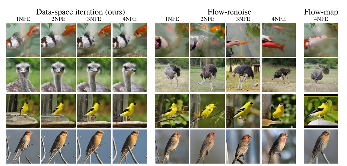
The picture that convinced me is Figure 2. Read across a flow-renoise row and the content changes at every call: in the goldfish row the scene goes from a pink blur to a goldfish, then to a hand holding a carrot, then to two red fish. Fresh noise is doing exactly what it was asked to. Each call keeps only what survives being mixed back to noise level , and at 0.75 that is not much. The data-space row keeps the same fish, in the same pose, and sharpens it.
The appendix puts a number on it. Table 6 measures the average L2 change between consecutive outputs over 50k samples, decoded to pixels in [0, 1]:
| change between calls | 1 → 2 | 2 → 3 | 3 → 4 |
|---|---|---|---|
| flow-renoise | 82.72 | 51.18 | 29.91 |
| data-space | 59.65 | 44.25 | 35.98 |
Flow-renoise changes the image more in the first two transitions, as the pictures show. The detail I did not expect is the last column: data-space moves more than flow-renoise between calls three and four, 35.98 against 29.91. The renoise sampler at is mostly polishing. The data-space generator is still doing real work at its last call, and its steps shrink slowly rather than collapsing. If you squint, that is the per-sample "step size" the introduction asked for, chosen by the network rather than by . But the paper does not measure it per sample or per region, and the motivating claim that "spatial regions with different frequency content might benefit from different forms of refinement" stays a hypothesis here. Figure 3 shows signed per-pixel differences that concentrate on edges and the subject for data-space and spread over the whole frame for renoise, which is suggestive, on four images.
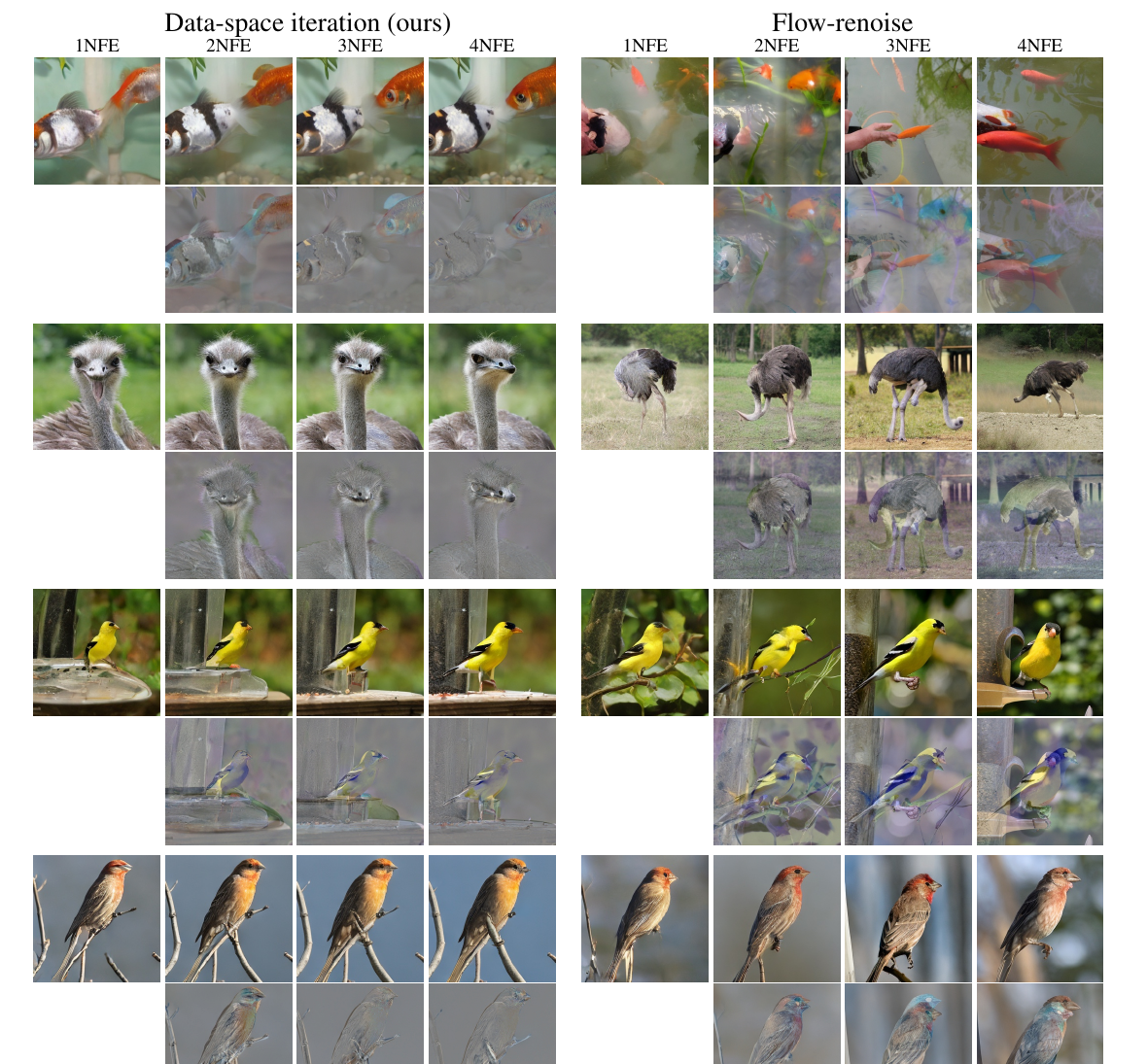
The full-metric table in Appendix C adds some texture to the FID story. At four steps without guidance, data-space has recall 0.59 against Phased DMD's 0.56, but lower precision (0.81 against 0.83) and a lower Inception Score (228.59 against 245.76). So the FID win comes from coverage more than from sharpness. That fits a generator that keeps its first composition, rather than one that gets three chances to land on a stereotypical class image. It is also the kind of trade-off that FID alone hides.
The one-step result is not evidence
At one call, data-space and flow-renoise are the same thing: one network evaluation from pure noise to an image. The paper says so in its CIFAR-10 appendix, and the CIFAR numbers show why to take the ImageNet one-step gap (3.85 against 4.45) with salt. On CIFAR-10 with a 55M UNet, data-space is worse at one step, 12.20 against DMD's 11.21. From two steps on it pulls well ahead, 8.28 against 11.14, and at four 8.62 against DMD's 10.03 and Phased DMD's 11.72. The authors attribute the one-step difference to optimisation dynamics and ask readers to judge the method at more than one step. I agree, and I would extend the caution a little: if optimisation alone can move one-step FID by more than half a point in either direction, a 0.02 gap at four steps is noise and an 0.08 gap is a lean, not a law.
One more oddity worth knowing: every distilled model here beats the unguided teacher by a mile, 2.46 to 2.75 against the teacher's 8.26. The paper credits DMD's reverse-KL objective, which is mode-seeking. It means unguided comparisons against the teacher flatter everyone. The guided teacher at 2.06 still beats them all, at about 125 times the calls of a four-step guided student (500 against 4).
Where it sits
The paper is careful about relatives, and I think the comparisons are fair.
Self-conditioning (Analog Bits and its descendants) also feeds the model its previous prediction. The difference is what the iteration is. Self-conditioning still integrates an ODE and uses the previous to improve the velocity at the next time; here the data estimate is the state and there is no ODE.
Deep equilibrium models solve for . Data-space iteration is not trying to converge: the step index changes the update, and the loss is applied at every step rather than at the fixed point. The failed optimal-transport regularizer is the experiment that tests the equilibrium intuition, and it loses.
Looped transformers reuse blocks to get depth, which makes them the closest relative of something this site covered last week, LiFT, which loops a DiT core inside each step and indexes loops with a continuous depth coordinate (the looped-transformer page has the background). Lin's own Adversarial Flow Models paper trained a looped generator end to end through the unrolled loop. Data-space iteration gets the loop without backpropagating through it: only one call carries gradients per training step. This is also why it drops into an existing DMD codebase without new memory tricks.
JiT came up in the replies, where someone asked whether this is the same idea as "Back to Basics", since both talk about data-space prediction. Lin's answer: "JiT's data prediction is designed to avoid the Transformer bottleneck, but it still operates within the probability-flow framework." I think he is right. JiT changes what one network call outputs; this paper changes what a sampler iterates on.
What I would do with it
If I were distilling a model with self-rollout today, especially a streaming video model where the schedule is baked into training, I would try this first. The reasons are practical. It removes a hyperparameter that the paper shows cannot be set by reasoning. It costs nothing at training time. It makes the model slightly smaller. Every prefix of the rollout is a usable image, so the step count can be picked at inference, up to the trained maximum. Lin's thread adds a recipe for large models: when an ODE-based initialisation is preferable, first consistency-distil to a one-step model, then apply data-space DMD.
What I would not do is read Table 3 as "data-space beats flow-map". Against a searched flow-map schedule it ties without guidance and leads by 0.08 with it. The evidence is one benchmark (ImageNet 256, class-conditional, one 675M backbone) plus a CIFAR-10 appendix, and the paper itself leaves text-to-image and video for future work, which is exactly where the motivation came from. The GAN and regression losses that production DMD stacks use were left out on purpose, so how the gain survives inside those is open. There is no code release beyond the two appendix algorithms, and no checkpoints.
The idea I expect to stick is the framing: the thing passed between calls is a design choice, and "a noisy image at a time someone picked" was never the only option.
How I checked
Everything in the paper sections comes from arXiv 2610.12102v1: the equations from §2, the training recipe from §3.1 and Table 4, the FIDs from Tables 1, 2, 3, 5 and 8, the step-to-step L2 numbers from Table 6, the code from Algorithms 1 and 2. Figures 1 to 3 are cropped from the PDF; the Table 3 image is the one Lin posted on X, which I compared against the HTML table cell by cell. I recomputed the parameter arithmetic (it adds up; 2,304 parameters of the timestep MLP's figure I could not attribute), the shifted schedules (they match Table 2(c)), and the 125× call ratio. The thread and replies came from the fxtwitter mirror of post 2109634731142787145. I looked for a code release on Lin's site and under the ByteDance-Seed and PeterL1n GitHub accounts and found none. The toy is my own numpy re-implementation of Algorithms 1 and 2 (single-threaded, about 100 seconds per run on a CPU), described in its section; its numbers are mine and say nothing about ImageNet.