2026-11-09 · 36 min · 3d · slam · realtime · feed-forward-reconstruction · long-video · visual-odometry
Why read this
Notabletop 60%Reads ABot-Recon's window, refiner and loop closure in code, and re-implements the cache, the pose chain, the composition loss and the pose graph on CPU.
- Interactive explanations
- Original analysis
- Concrete numbers to act on
3D & spatialNeeds datacenter GPUsMixed licencesResearch paper
How this was scored
- Is it new?
- 1 of 3: An incremental tweak
- Can I trust it?
- 2 of 3: Measures key facts from files, code or configs
- Can I run it?
- 1 of 3: API-only, gated or restrictive licence
- Will I understand it?
- 3 of 3: Mechanism carried by interactives built from real code or data
- Can I act on it?
- 2 of 3: A concrete recipe, numbers or comparison
- Will it last?
- 1 of 3: Relevant for months
- Does it affect many?
- 1 of 3: A specialist community
- Only here?
- 2 of 3: A teardown or measurement few others did
Score 60 of 100, ranked 395 of 701 rated articles. Each question is answered 0–3 by hand, and a 3 is rare. How articles are scored
A post on X pointed at ABot-Recon, a streaming 3D reconstruction model from Alibaba's AMAP CV Lab that "doesn't need to keep the entire video history inside a growing attention window". The paper is arXiv 2608.27529, "Revisiting Local Context for Long-Horizon Streaming 3D Reconstruction". The code is at amap-cvlab/ABot-Recon and the checkpoint at acvlab/ABot-Recon on Hugging Face. There is a project page too. It is the same lab as ABot-World-0, which this site took apart in August.
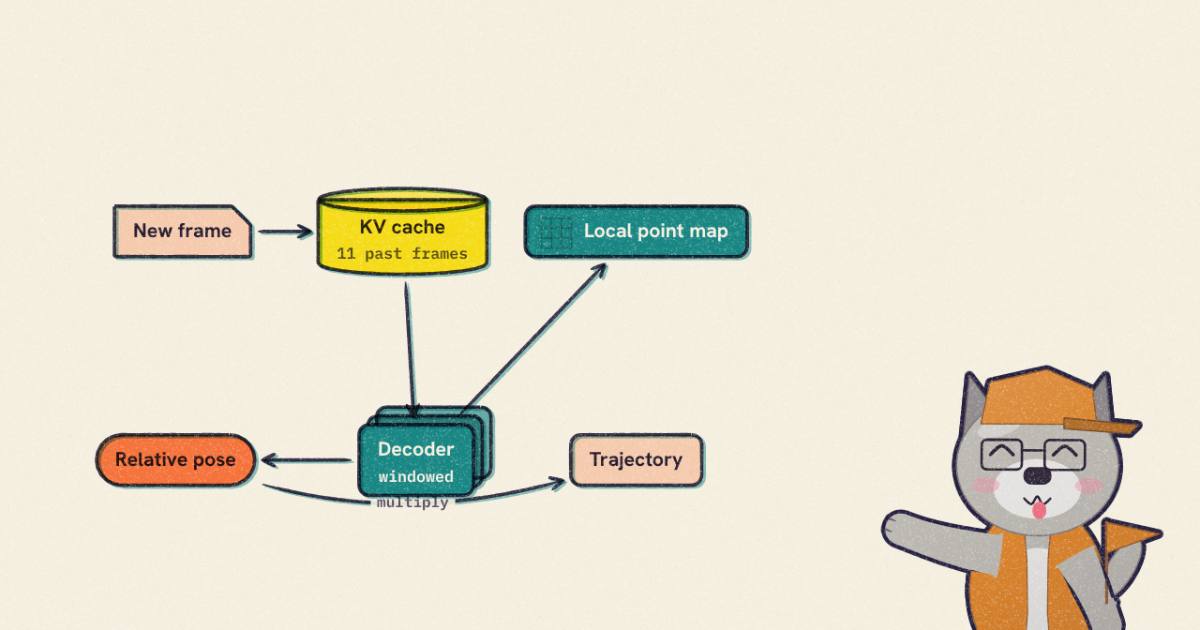
The claim is easy to state. The model reads each new frame once, attends to the 11 frames before it and nothing older, and still tracks the camera over 18,846-frame drives. This site has covered the other way to get there. R³ and AMB3R-SLAM keep keyframe banks and pose graphs, and HiP3R stitches chunks with two graphs after the fact. ABot-Recon's answer is that most of that state is unnecessary if you change what the network is asked to predict.
What I did, and how each claim below is labelled:
- Reported: a number from the paper or the README that I did not re-run.
- Read: something I saw in the released source at commit
6e3b2e1(15 October 2026) or in the checkpoint's safetensors header, which I fetched with an HTTP range request. I did not execute the authors' code: the sandbox refused to import the repository's modules, even its torch-only cache and mask files. - Measured: output of my own scripts, run on this box's CPU with 2 threads.
toy.py(torch 2.14.1) covers the cache, the rotary positions and the pose chain;composition.pythe composition-aware loss; andloop_closure_toy.pythe loop-closure back end. The last two are numpy 2.5.4 only and sharelie.py. Each re-implements a piece of the mechanism from what I read. None of them is the model, and none ever sees an image. - Reasoned: arithmetic on the other three.
The problem: long video breaks streaming models in two ways
Feed-forward geometry models (DUSt3R, VGGT, π³) predict cameras and point maps for a set of images in one pass. To run one on a video you make it causal: frame attends to frames before it, and you keep their keys and values in a cache so they are not recomputed. That is StreamVGGT's design. It has two costs that grow with the stream.
The first is memory. Every frame's keys and values stay in the cache, so a video twice as long needs a cache twice as big and attention twice as wide.
The second is the prediction target. If every pose is expressed in the first frame's coordinates, then the network at frame 4,000 is asked to say where it is relative to a view it saw minutes ago. The paper's framing is that the target's "estimation range grows with the sequence" (reported). A model trained on 32-frame clips has never seen that range.
The field's recent answers add memory back in a managed form. LingBot-Map keeps anchor frames, a pose-reference window and a trajectory memory; HorizonStream couples local attention with persistent linear attention; CUT3R and TTT3R carry a recurrent state (reported, the paper's related work). ABot-Recon removes the long-range state instead.
The idea: predict only local things, then chain them
For each incoming frame the model outputs three things (reported, Section 3.1):
- a point map in the current camera's coordinates,
- a confidence map ,
- one relative pose from the current camera to the previous one.
None of those depends on how long the stream has been running. A point map in the current camera is the same task at frame 10 and at frame 10,000. So is the motion between two adjacent frames. The global trajectory is never predicted; it is computed, by multiplying the relative poses together:
and each local point map is moved into the world with its frame's composed pose. That is ordinary visual odometry. The new part is doing it with a learned feed-forward model whose own context is fixed, and training it so the chain does not fall apart.
The network, with shapes
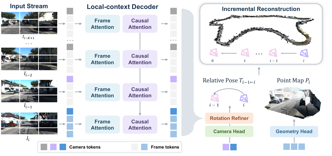
The backbone is π³'s. The released network is built on its code (abot_recon/modeling/pi3/), and training starts from
π³'s public weights (read and reported). Here is one frame's path through it at the paper's 504 × 280 input, with
every shape taken from the source (read, pi3.py, network.py, adjacent_pose_head.py, commit 6e3b2e1).
- Encoder. DINOv2 ViT-L/14 with registers (
dinov2_vitl14_reg). 14-pixel patches make 36 × 20 = 720 patch tokens of width 1,024. The encoder sees one frame at a time, so it has no memory at all. - Decoder. Five learned register tokens are prepended, making 725 tokens a frame. Then 36 blocks of width 1,024 with 16 heads of 64. Even blocks attend within the frame. Odd blocks attend across frames, through the 12-frame window below. Only those 18 odd blocks keep a cache.
- Fork. The outputs of the last two decoder blocks are concatenated, 2,048 wide, and handed to three small decoders: points, confidence and camera.
- Geometry head. A linear head per 14-pixel patch unfolds each token into a 14 × 14 patch of three numbers, . The point is in the current camera, so depth is predicted in log space and the ray direction is scaled by it. That is , and the confidence head gives the same way.
- Camera head. The five register tokens double as camera tokens; the camera decoder leaves them 512 wide. Each goes through a two-layer MLP and the five are averaged: that is in the paper's Equation 2. The pair descriptor of Equation 3 is
The four blocks let a two-layer MLP see both frames, their difference (what moved) and their product (what agrees) without having to learn subtraction. That MLP returns 512 numbers, and two linear layers turn them into a translation and a scalar-last quaternion, normalised into a rotation . The quaternion format is enforced: the head raises an error for any other (read).
The relative pose for frame is then
where is the rotation refiner's axis-angle correction (Equation 11), applied on the
right, inside the step, before anything is chained. In the code the running pose is one matrix product per frame:
current_pose = previous_pose @ corrected_delta (read). The only state the camera head carries from frame to frame
is the previous descriptor, the previous frame's tokens, that running pose and the refiner's buffer of 10 pair
features. All of it is fixed-size.
How memory stays bounded: a 12-frame band, enforced in code
The post's heading is "Only 12 frames of local context". That is literal. InferenceConfig raises
ValueError("The released model requires a 12-frame local window") for any other value, and the attention mask in
core/window_mask.py blocks key frame for query frame when or when is more than
11 (read). The cache that feeds it, StreamingKVState.append_committed_frame, keeps at most 11 past frames: once
full, it shifts the buffer left and writes the new frame into the last slot. The comment above that shift records a bug
they hit: an overlapping in-place copy_ "silently corrupts older window entries on CUDA" (read).
Two things in the code are more interesting than the band itself.
The hooks for long-range memory are there, and switched off. The cache classes take num_reference_frames (frames
pinned forever, like LingBot-Map's anchors) and num_summary_tokens (a few tokens of every evicted frame, kept as a
compressed history). The released constructor passes neither, so both default to 0 (read, model.py and
network.py). The paper's claim of "no persistent learned long-range state" is a configuration of a codebase that
could carry one. My guess is that the authors tried the anchors and summaries and found them unnecessary; the paper
does not report that experiment (reasoned).
Positions are absolute, attention is not. The rotary embedding on the frame axis uses each frame's absolute index,
"kept for 3D rotary positions even after older frames leave the window" (read, kv_state.py). Rotary embeddings
make a query-key score depend only on the difference of positions, so frame 20,000 attending to frame 19,995 should see
exactly what frame 11 sees attending to frame 6. The angle table is built in float64 and has max_seq_len rows, set to
max_frames, 22,000 by default (read). I rebuilt the frame-axis rotation (20 of the 64 head dimensions, θ = 10,000)
and compared scores at frame 11 and frame 20,000 for the same offsets (measured): in fp32 the largest difference
over 725 × 725 scores was 7.6e-6, against a mean score magnitude of 3.5; in bf16 it was 0.15, the same size as bf16's
own error at frame 11 (0.11 to 0.15 against a float64 reference). The window's attention loses nothing to a late position. The one
practical consequence is a cap: a stream longer than --max-frames would index past the table, so a 30,000-frame drive
needs the flag raised (reasoned; I did not run past it).
How big the cache is, and what 6.71 GiB buys
The paper reports 24.45 FPS and 6.71 of peak GPU memory on KITTI-02 at 504 × 280 on an H100, "input storage excluded" (reported, Table 6). The table does not give the unit and the text says "6.71 GB". PyTorch's peak-memory counters are usually divided by and printed as "GB", so I read it as GiB below; if it is decimal gigabytes it is 6.25 GiB, and the unexplained remainder further down shrinks from 1.6 to 1.1 GiB (reasoned). I wanted to know how much of it is the window.
At 504 × 280 with 14-pixel patches a frame is 36 × 20 = 720 patch tokens plus 5 register tokens, 725 in all. Each of the 18 cross-frame layers stores a key and a value for each, 16 heads of 64, in bf16 (read: the paged path casts to bf16 because FlashInfer will not take fp32). That is 18 × 2 × 725 × 1,024 × 2 bytes = 53,452,800 bytes, 50.98 MiB per frame (reasoned).
So the 11-frame window holds 0.548 GiB. The paged allocator reserves 28 frame pages (the window of 12 plus 16 spare), 1.394 GiB, once, at the start (read and reasoned). The checkpoint is 1,000,934,176 parameters, all float32 in the file, 4.0 GB, which I read from its header without downloading it; nothing in the loader casts them, and inference runs under bf16 autocast (read). Weights at 3.73 GiB plus the 1.394 GiB pool is 5.12 GiB; the remaining 1.6 GiB of the reported peak is activations and FlashInfer's 128 MiB workspace (reasoned, not profiled). The window is about a fifth of the memory.
Had the cache kept everything, KITTI-02's 4,661 frames would need 232 GiB of keys and values, and VBR's 18,846-frame Ciampino-1 drive 938 GiB (reasoned). A plain full-history cache is not an option at these lengths on any single GPU.
My toy shows the shape on a CPU (measured, one attention head, 64 tokens of width 64 per frame). With a 12-frame window, a frame costs 0.31 ms at frame 12 and 0.18 ms at frame 3,000. With a cache that keeps everything it costs 1.3 ms at frame 100, 21 ms at frame 1,000 and 113 ms at frame 3,000. The toy says nothing about H100 throughput; it says the window's per-frame cost is flat and the full cache's is not.
What is not bounded
The post is right that "storing the resulting point cloud still requires space proportional to the amount of
reconstructed geometry". The code makes that concrete. inference_stream_iter appends each frame's outputs to a Python
list and concatenates them at the end, with no move to the CPU inside the loop (read). A local point map at
504 × 280 is 1,693,440 bytes in fp32 and its confidence map 564,480 bytes, so dense outputs for all of KITTI-02 come to
about 10.5 GB (reasoned). The README's --dense-stride N and the API's dense_output_indices are the escape hatch:
poses for every frame, dense geometry for a subset. Use them on long runs.
The optional loop closure is not bounded either, by design. It retrieves revisited frames with DINOv2-SALAD descriptors
and FAISS, then re-runs ABot-Recon on windows centred on both frames to get a relative pose, so it needs the old images
and a descriptor per keyframe (read, loop_closure.py, and reported, Section 4.1).
The price of a short memory: drift, and why rotation gets the fix
A chain of relative poses drifts. Every small error stays in the product forever. The paper's two additions are aimed at exactly this, and the toy below shows why they aim at rotation.
I composed 4,661 noisy relative poses along a synthetic drive the size of KITTI-02 (1.094 m a step, 12 random 90-degree turns), aligned the result to ground truth with a Sim(3) fit as the paper does, and averaged eight seeds (measured).
Translation noise of 5% of every step gives an ATE of 2.03 m. A heading error of 0.05° per step, with no translation noise at all, gives 13.3 m; at 0.1° it is 26.57 m (measured). A wrong step length is one wrong step. A wrong heading turns every step after it, so the error grows with distance travelled. Over a gap of 11 frames the 0.05° chain is off by 0.534 m; over 1,000 frames by 26.6 m (measured). The toy's noise levels are mine, chosen to show the shape, not estimates of the model's errors.
The paper's two fixes are the same diagnosis in network form.
The rotation refiner, read line by line
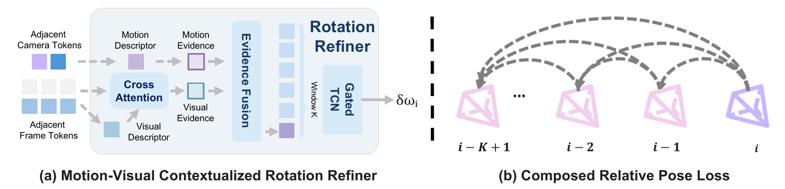
The paper describes a module that takes the pairwise camera descriptor, adds visual evidence by cross-attending from a pooled frame-pair query into both frames' dense tokens, then runs a gated temporal convolution over recent pair features to predict a small axis-angle correction to the relative rotation. Translation is left as predicted (reported, Section 3.3). In symbols, with the fused pair feature:
proposes a hidden vector from the window, proposes a gate in for each channel, and maps the
gated result to three numbers. The source is more specific than the notation, in three ways (read,
TemporalRotationRefiner in adjacent_pose_head.py and RELATIVE_CAMERA_HEAD in model.py).
- The window is 10, not 12. The feature buffer keeps the last 10 pair features, padded with zeros at the start of a
stream, and a learned
age_embedis added to each slot so the network knows how old a feature is. - The "TCN" is one depthwise convolution.
convandgateareConv1dlayers withgroups=512and kernel 10, run over a 10-long buffer with no padding. Each produces exactly one output step. So is, per channel, a learned weighted sum of that channel's last 10 values; is another, through a sigmoid. It is a gated linear filter over time, one per channel, not a stack of dilated layers. - The correction is clamped. is a single linear layer to three numbers, then
max_rad * tanh(...)withmax_rad= 2.0°. Each axis-angle component is at most 2.0 degrees, so the refiner can trim a step but never rewrite one.
I wanted to know where the 4.75 million parameters sit, so I rebuilt the module's layer list from the source with hidden width 512, a 512-wide camera token and 8 attention heads, and counted (reasoned from the code, then checked against the checkpoint):
| Piece | What it does | Parameters |
|---|---|---|
desc_proj | LayerNorm(2,048) and a two-layer MLP on the motion descriptor | 1,315,840 |
frame_query_proj | the same shape, on the pooled frame pair | 1,315,840 |
frame_proj + role embedding | projects both frames' tokens into the attention's key space, tags which frame | 263,680 |
frame_attn + frame_norm | one 8-head cross-attention from the pair query into both frames' 1,440 patch tokens | 1,051,648 |
fuse_proj | LayerNorm(1,024) and a two-layer MLP: motion plus visual evidence into | 789,504 |
age_embed | one 512-vector for each of the 10 slots | 5,120 |
conv + gate | the two depthwise temporal filters | 11,264 |
out | linear to the three-number residual | 1,539 |
| total | 4,754,435 |
The total matches the checkpoint's 4,754,435 to the parameter (read, safetensors header), so this is the released module and not a near relative. The part the paper names, the temporal convolution, is 11,264 parameters, 0.24% of the refiner. Almost all of the refiner is evidence-building: two pair MLPs and one cross-attention, so that each step gets a compact feature that already says how much the camera turned and what the pixels say about it. The temporal part is small because its job is small: weigh the last 10 of those features. Its state is a 10 × 512 buffer, so it does not break the memory bound.
One thing the refiner never sees is its own past output. The buffer holds fused features, not past corrections or past composed rotations. It can learn that a run of features looks like a turn, but not that the last five corrections all leaned left (read and reasoned).
The composition-aware loss, term by term
Training does not only supervise each adjacent pair. For a clip of frames the supervised set is every pair at most frames apart (reported, Equations 12 to 14):
For each pair the predicted adjacent poses between and are multiplied out (Equation 5) and compared with the true . Rotation is weighted by the gap:
Reading it term by term. and are π³'s translation and rotation losses, applied to the
composed transform. The denominator of makes the weights average to 1, so moves weight between
gaps without changing the loss's scale. makes the weight grow slower than the gap. Translation is not
weighted at all. A separate term, , penalises the size and the frame-to-frame change of the
refiner's residuals (reported, Equation 15). The paper does not give , the s, or the exact forms of
; the train branch has the training code and I did not read it.
Two consequences fall out of the definition (reasoned, checked in the second tab of the widget below). First, most of the rotation weight is on long gaps: at in a 128-frame clip, adjacent pairs are 9.5% of the pairs but carry 4.1% of the rotation weight. Second, and this corrects my first version of this article, a longer clip does not contain longer chains to grade. caps the gap at 11 whatever is. A 128-frame clip has 1,342 supervised pairs and a 32-frame clip 286, with nearly the same mix of gaps. What 128 frames add is more pairs per clip and fewer clip boundaries, which is the paper's own explanation of its ablation.
Experiment: what the composition loss can see
The point of grading chains is that some errors only show up in a chain. An adjacent-pair loss scores each step on its own. If two predictors make the same size of error per step, it cannot tell them apart, even when one predictor's errors all lean the same way and the other's cancel. Their trajectories are very different.
I tested exactly that (measured, composition.py). Each step's rotation error is an AR(1) process,
, scaled so the per-step spread is 0.05° per axis for every . Only
the step-to-step correlation changes. For each I computed the adjacent-pair rotation loss (geodesic angle), the
rotation term of above on random 128-frame clips with and , and the
Sim(3)-aligned ATE of the whole 4,661-frame drive, over six seeds.
| ρ | adjacent loss | composed loss | ATE |
|---|---|---|---|
| −0.5 | 0.080° | 0.130° | 7.06 m |
| 0 | 0.080° | 0.203° | 12.25 m |
| 0.5 | 0.080° | 0.313° | 21.32 m |
| 0.9 | 0.080° | 0.479° | 54.37 m |
| 0.98 | 0.078° | 0.523° | 120.65 m |
The adjacent loss is flat at 0.08° across a 17-fold range of ATE. A model trained only on it has no gradient toward the better trajectory. The composed loss tracks the ATE from to , so a model trained on it is pushed toward errors that cancel. That is the paper's ablation in miniature: the composition loss alone took KITTI's ATE from 56.60 m to 27.66 m.
The last row is the catch. From to the ATE more than doubles while the composed loss moves from 0.479° to 0.523°. An AR(1) error with stays correlated for about 50 frames, and the loss looks at most 11 frames back. Error that leans the same way for longer than the window, such as a slow calibration bias or a long gentle curve the model consistently under-turns, is invisible to the loss that is supposed to catch drift. Nothing in the 12-frame model sees it either; that is what loop closure is for (reasoned).
Negative correlation is the other lesson. At the ATE is 7.06 m against 12.25 m for independent errors at the same per-step size. A refiner that looks at the last 10 pair features can learn to lean against a recent run of errors, and the composed loss rewards that. Whether the trained refiner does so I cannot say without running it.
What the ablation says
The ablation in the third tab of the drift widget says the loss did the most work: on KITTI, adding it alone took average ATE from 56.60 m to 27.66 m, training on 128-frame clips instead of 32 took it to 22.31 m, and the refiner to 18.25 m (reported, Table 8). Every row keeps the 12-frame window. Clip length during training mattered even though neither the window nor the longest supervised chain changed. The paper's reading is more data per clip and fewer artificial clip boundaries; I agree, with one caveat: the paper does not say whether the ablation rows were trained for the same number of steps, and its main recipe's 128-frame stage is a second stage started from the first, so the row may mix clip length with extra training.
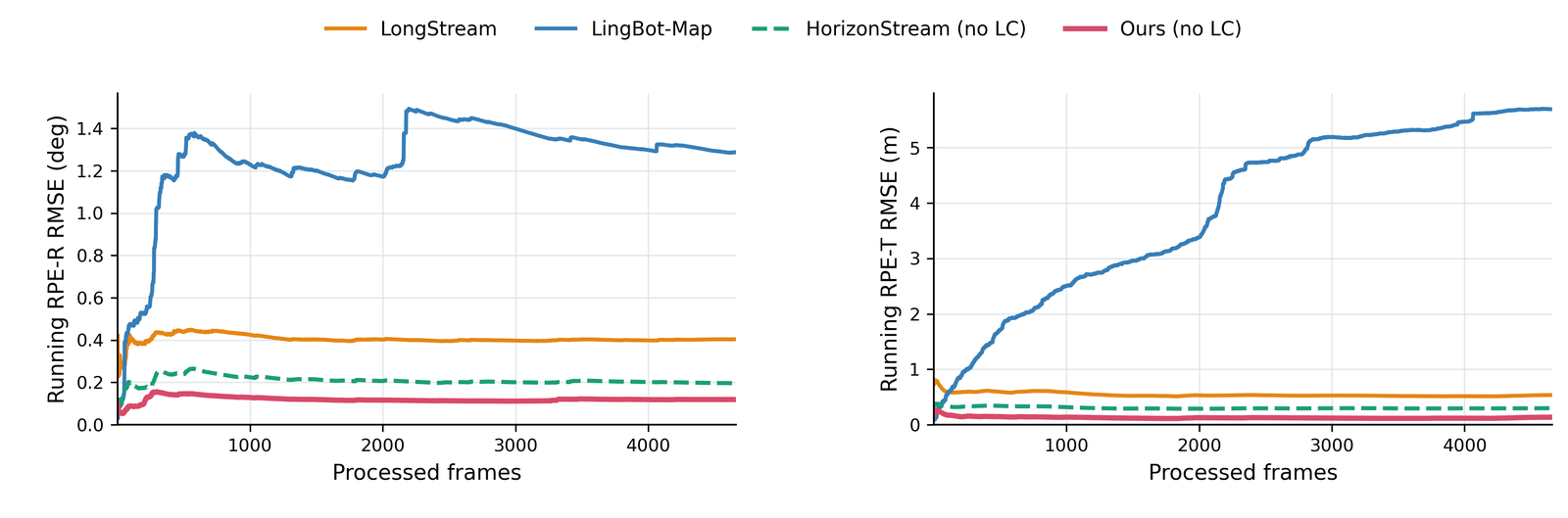
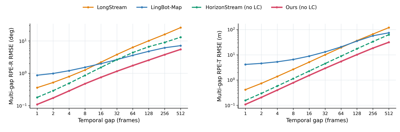
The paper's own diagnostic shows the result: adjacent-frame error that stays flat across a 4,661-frame sequence, and multi-gap error that grows more slowly than the other streaming models'.
The results, read against their own tables
All of this section is reported (Tables 3 to 7) unless marked.
KITTI (11 sequences, 271 to 4,661 frames): average ATE 18.25 m without loop closure, the lowest in the table; the next streaming model is HorizonStream at 22.51 m, and the best optimisation-based entry is SLAMFormer-∞ at 23.01 m, quoted from its own paper. With loop closure, 13.49 m against HorizonStream's 17.98 m. Per sequence it is not a sweep: on 02, the longest, 69.87 m against HorizonStream's 97.24 m, but on 06 it is 12.04 m against HorizonStream's 5.46 m.
Oxford Spires (10 sequences of about 3,840 frames): ATE 4.35 m and RPE-R 0.12°, the abstract's "approximately 40%" better than the best prior results. That is against streaming methods: LingBot-Map's 7.32 m and HorizonStream's 0.20° (reasoned: 4.35 / 7.32 is 40.6% lower, 0.12 / 0.20 is 40% lower). It is not the best number in Table 4. DPVO reaches 1.56 m, Droid-W 2.27 m and DPV-SLAM 2.95 m, and Droid-W's RPE-R is 0.08°. The paper says so and points out that those three need camera intrinsics while ABot-Recon reads only RGB. That is a fair distinction, and it is also the honest headline: on this benchmark a classical-style optimiser that knows its camera still wins.
VBR (7 sequences, 8,815 to 18,846 frames): without loop closure, 30.14 m, behind HorizonStream (29.02 m) and LingBot-Map (29.45 m). The paper calls that "competitive", which is accurate. With loop closure it drops to 9.99 m, the lowest in the table, against HorizonStream's 17.64 m with its own loop closure.
Dense reconstruction: on Oxford Spires, Chamfer distance 1.37 m and F1 91.81% at a 4 m threshold, the best of the nine streaming methods (LingBot-Map 1.68 m and 90.58%). On 7Scenes, F1 94.88% against HorizonStream's 98.22% and LingBot-Map's 96.01%; on TUM-Dynamic, 92.19% against LingBot-Map's 95.97%. The paper's discussion concedes the indoor gap and suggests compact scenes, with lots of revisiting, are where persistent memory still pays.
Speed: 24.45 FPS and 6.71 GiB, frame by frame on one H100. CUT3R (29.62 FPS, 3.16 GiB) and TTT3R (25.53 FPS, 4.65 GiB) are faster and smaller, and drift far more: CUT3R's KITTI ATE is 209.04 m. LingBot-Map takes 18.87 GiB and HorizonStream 13.04 GiB in the same mode.
Two protocol notes. Every trajectory is aligned to ground truth with a Sim(3) Umeyama fit before ATE, so scale is free; a monocular model's metric-scale error is not in these numbers. And the training mixture includes KITTI-360 and Waymo (reported, Table 1), which are driving data close to KITTI's domain but not its test sequences.
Loop closure, read and re-implemented
Everything above is the streaming model alone. The best numbers in the paper are not. On VBR, loop closure takes ATE from 30.14 m to 9.99 m, and on KITTI from 18.25 m to 13.49 m (reported, Tables 3 and 5). It is a separate, training-free back end, and its code is worth reading, because the bounded-memory story stops at its door.
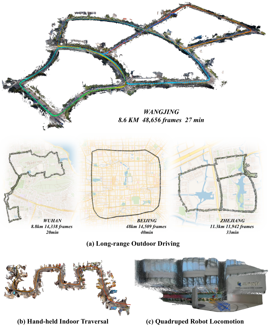
Where it helps on KITTI is a list of the sequences that revisit places (reported, Table 3): 00 goes from 21.86 m to 11.70 m, 02 from 69.87 m to 39.00 m, 05 from 13.54 m to 6.00 m and 06 from 12.04 m to 8.70 m. Sequences 01, 03, 04, 08 and 10 do not change at all. 08 is the interesting zero: it does revisit streets, but in the opposite direction, and a forward-facing camera sees a different picture going the other way, so appearance-based retrieval is unlikely to match them (reasoned; the paper does not discuss it).
What the code does
The pipeline in loop_closure.py and sparse_loop/ runs after the stream, on the whole trajectory (read,
defaults in LoopClosureConfig):
- Describe every frame. DINOv2-SALAD descriptors at 336 × 336, one per frame (
keyframe_stride1). In the demo they are computed by a worker thread while the stream runs. - Retrieve. FAISS inner-product search, top 5 neighbours per frame. A pair survives if its score exceeds 0.85 and the two frames are more than 30 frames apart.
- Suppress. Candidates are ranked by score and kept greedily; each kept pair blocks every other candidate within 25 frames of either end. At most 50 survive to the next step.
- Measure. For each pair, the 10 frames centred on each end are put in one list, sorted by index, and run through ABot-Recon as a single 20-frame stream. The relative pose between the two centre frames is read off that stream's chained poses.
- Optimise. A sparse SE(3) pose graph: a node every 50 frames plus every loop endpoint, an odometry edge between consecutive nodes from the streamed trajectory, one edge per loop. Levenberg-Marquardt for 30 iterations, first node fixed, on CUDA only (the solver raises without a GPU).
- Spread. Each node's correction is interpolated to every frame between nodes: rotations by slerp, translations linearly.
Four details matter more than they look.
The loop measurement asks the model to do something it was not trained for. In step 4, with the old frame and the new one, frame is followed directly by frame . To the model that is one adjacent step, and the relative pose between the two visits rests on that one prediction across a jump of thousands of frames. It works when the two visits look alike, which is what retrieval selected for, and the 30-frame and 25-frame rules keep it from being asked about the same place twice in a row (read and reasoned).
Every loop edge gets the same, small weight. The weight is
pose_graph_loop_weight * sqrt(inliers / rigid_min_inliers), 0.01 × √(128 / 24) = 0.0231. But inliers is never
counted: every edge is created with the config's default_inliers, 128. There is no per-edge verification, and the
graph has no robust kernel. Odometry edges get weight 1, and since the residual is multiplied by the weight before it
is squared, one loop edge counts for about 1/1,875 of an odometry edge (read and reasoned).
SE(3), not Sim(3). The graph's pose_graph_model defaults to se3 and the loop config does not change it. A
monocular chain can drift in scale as well as in pose; this back end can bend the trajectory but cannot rescale part of
it (read).
Rotation and translation share a scale. Both residual weights are 1.0, so one radian of rotation error costs the same as one metre of translation error.
Experiment: the released back end on a drive that comes home
I re-implemented steps 3, 5 and 6 with the released defaults: the NMS rule, the keyframe stride, the edge weights, the
residual on world-to-camera log coordinates, the
Levenberg-Marquardt schedule (λ from 1e-6, halved on success, doubled on failure) and the slerp spreading
(measured, loop_closure_toy.py). Steps 1, 2 and 4 need the model and SALAD, so I stood in for them: a candidate
is any frame within 4 m of an earlier frame at least 31 frames back, scored by distance, and each loop measurement is
the true relative pose with 0.05° and 0.05 m of noise. That makes my loop edges better than the real ones can be.
The drive is 4,661 frames, the length of KITTI-02: a 1,300 m × 900 m loop, then 640 frames back over its own start, like KITTI-00. The streamed trajectory has 0.05° of rotation noise and 2% of translation noise per step. The retrieval rule finds 642 candidate frames on the revisit; NMS keeps 20, below the cap of 50. Four seeds.
| Setting | Loop edges | ATE |
|---|---|---|
| no loop closure | 0 | 15.68 m |
| released weight | 20 | 5.10 m |
| weight × 10 | 20 | 4.00 m |
| weight × 100 | 20 | 3.74 m |
| released weight | 1 | 7.52 m |
| released weight | 5 | 5.57 m |
| weight × 100 | 1 | 4.19 m |
| released weight, plus one false loop | 20 + 1 | 58.65 m |
| weight × 100, plus one false loop | 20 + 1 | 313.87 m |
Three readings (measured, then reasoned).
It works, and it is cautious. The released setting cuts this drive's ATE by two thirds, 15.68 m to 5.10 m. Raising the loop weight a hundredfold gets 3.74 m. With good edges the low weight leaves about 1.4 m on the table.
One edge does most of it. A single loop edge at the released weight gets 7.52 m; five get 5.57 m; twenty get 5.10 m. A revisit's edges all say much the same thing, which is why NMS can afford to keep few of them.
One false loop costs more than all the true ones save. I added a single wrong edge, frames 2,300 and 900, which are 920 m apart, measured as "the same place": two intersections that look alike. At the released weight the ATE goes from 5.10 m to 58.65 m, nearly four times worse than not closing loops at all. At a hundred times the weight it is 313.87 m. The small weight is the only defence the graph has, and it limits the damage rather than preventing it. In the released pipeline, everything rides on the 0.85 SALAD threshold and the model's re-inferred pose being right.
The paper's KITTI and VBR rows show no such failure, so retrieval held on those sequences. For a fleet of drives through repetitive streets, I would add a check before trusting an edge: the re-inferred relative pose against the odometry's own estimate, or the point maps' overlap, which the code already has (reasoned).
And the memory bound does not cover it. Step 4 reads the old images back from disk, and steps 1 and 2 keep one descriptor per frame. That is optional and offline, and it is linear in the length of the drive (read).
Training cost, licence and running it
The recipe, all reported (Section 4.1 and Tables 1 and 2):
| Stage | Clips | Iterations | Hardware | What trains | Peak learning rate |
|---|---|---|---|---|---|
| I | 32 frames | 32K, batch 48 | 48 NVIDIA H20 | everything but the confidence branch; the absolute camera output is replaced by the adjacent-pose head | 1e-4, annealed to 1e-6 |
| II | 128 frames | 38K, batch 32 | 32 AMD MI308 | everything, refiner switched on | 5e-5 for the refiner, 2e-5 for the rest |
| III | as II | 4K | not stated | confidence branch only | 2e-5 |
AdamW throughout, an EMA of the weights with decay 0.999, bf16 mixed precision, gradient clipping at 1.0, one sequence
per GPU. Images are resized to width 504 and centre-cropped or padded to 504 × 280. The data mixture is 30 datasets,
62.05% synthetic by sampling weight (TartanAir and TartanAir-v2, OmniWorld-Game, VirtualKITTI2, HyperSim and others)
and 37.95% real (DL3DV, Waymo, ScanNet++, KITTI-360 and others, plus unnamed internal data). Unordered multi-view sets
are turned into pseudo-videos by walking a camera pose graph. The appendix also shows rejected samples: sideways and
upside-down BlendedMVS images and broken TartanAir and OmniWorld scenes, which is a useful reminder that a large mixture
needs cleaning. Fine-tuning code is on the repository's train branch (read, README).
The split learning rate in Stage II is the detail I would copy. The refiner starts from scratch, with its output layer
initialised to zero, so its first correction is exactly nothing (read, reset_parameters), on top of a backbone
that already predicts good steps. A lower rate for the backbone stops the new
module's early, noisy gradients from undoing Stage I (reasoned).
The licences need care. The source code is Apache-2.0. The weights are not: MODEL_LICENSE.md puts them under CC BY-NC
4.0, non-commercial research and education only, because they are derived from π³'s weights, and says commercial use
"requires separate written authorization from all relevant rights holders" (read). The Hugging Face model card's
metadata says license: apache-2.0, which contradicts the repository's own file; I would go by the more specific
statement and treat the weights as non-commercial.
The released setup targets Linux, Python 3.10 or later, PyTorch 2.5.1 and CUDA 12.1, with FlashInfer for the paged cache and an SDPA fallback without it (read). The network has a CPU branch, but it would load 4.0 GB of fp32 weights and run a 1B-parameter model per frame, so I did not try. There is a hosted demo on Hugging Face Spaces and ModelScope, and a community port to the Axera AX650N NPU (read, README).
pip install torch==2.5.1 torchvision==0.20.1 --index-url https://download.pytorch.org/whl/cu121
pip install -e .            # inside a clone of amap-cvlab/ABot-Recon
pip install flashinfer-python   # optional: paged KV cache
python demo.py --image-dir frames/ --output-dir out/ --no-loop-closure --dense-stride 10- license
- Apache-2.0
- branch
- main
- tests
- 14 files
- source
- 593.8 kB
- commit date
- 2026-10-14
by size of tracked source at this commit, file counts in brackets; docs, data and vendored trees excluded
local clone, 2026-11-10 at 6e3b2e1 — branch, commit, commitDate, fileCount, hasTests, languages, license, licenseFile, shallow, testFileCount
shallow clone: counts describe the pinned tree, not the history
- architecture
- abot_recon
- task
- image-to-3d
- license
- apache-2.0
- safetensors
- 1 shard
- largest file
- 4.00 GB
- files
- 4
- downloads
- 1.9K
- likes
- 28
repo last modified 2026-09-01
Where it sits
The streaming 3D reconstruction literature has spent two years adding memory back to feed-forward models. CUT3R and TTT3R carry a recurrent state; StreamVGGT keeps the full causal cache; LingBot-Map keeps anchors, a pose-reference window and a trajectory memory; HorizonStream pairs local attention with persistent linear attention (reported, the paper's related work). On this site, R³ and AMB3R-SLAM keep keyframe banks and optimise pose graphs online, HiP3R reconstructs chunks and stitches them with two graphs, and StructureGS-SLAM closes drift against walls rather than loops.
ABot-Recon is the opposite bet, and it is the classical one. Visual odometry has always predicted adjacent motion and chained it; DPVO and DROID-SLAM do it with a learned matcher and a bundle adjustment over a sliding window, and add a pose graph for loops. ABot-Recon replaces the matcher and the window optimiser with one feed-forward network that never optimises anything at inference, and keeps the pose graph as an optional extra. That is why its comparisons split the way they do: against the memory-heavy streaming models it wins on long drives, and against the classical optimisers with known intrinsics (DPVO, DPV-SLAM, Droid-W) it loses on Oxford Spires (reasoned from Tables 3 to 5).
The broader overviews are in the site's 3D reconstruction roundup.
What I did not check
- I did not run the model. The sandbox refused to execute the repository's code, and the model is 4.0 GB of fp32 weights with a CUDA-first runtime. Every benchmark number above is the paper's.
- The 50.98 MiB per frame and the 1.6 GiB of activations are arithmetic from tensor shapes and the reported peak, not a profile.
- My first drift toy uses Gaussian noise that is independent from step to step.
composition.pyadds correlation and shows how much it matters (12.25 m to 54.37 m at ), but the correlation structure of the real model's errors is unknown to me. I did not measure it. composition.pyevaluates the loss; it does not train anything. Whether a network trained on the composed loss actually learns anti-correlated errors is the paper's Table 8 claim, not something I reproduced. I also had to pick (0.5); the paper does not publish it.loop_closure_toy.pyuses true positions in place of SALAD retrieval and near-true loop measurements in place of the model's re-inference, and its drift has no scale component, so the SE(3) graph's inability to fix scale never shows. Its numbers are an upper bound on what the released back end can do with good edges, and a demonstration of what one bad edge costs. My solver uses numerical Jacobians and a dense solve where the released one uses PyPose Jacobians and a preconditioned conjugate gradient on CUDA; on a graph of this size both should reach the same minimum, but I did not run theirs.- I did not read the
trainbranch, so the training-loss details (γ, the λs, the exact π³ losses) are the paper's description only. - I did not verify that the released checkpoint is the one behind Tables 3 to 8. The checkpoint's parameter counts match the paper's (1B in total, 4.75M in the refiner).
Verdict
ABot-Recon is a clean result: a feed-forward model with a fixed 12-frame view, no anchors, no compressed history and no recurrent state, which beats the long-memory streaming models on KITTI and Oxford Spires and ties them on VBR. The memory bound is real and enforced in code, at about half a gibibyte of window on top of the weights. The insight that makes it work is about targets, not caches: ask only for things that look the same at frame 10 and frame 10,000, then spend the training budget on making their product hold together, mostly the rotation. My CPU re-implementations agree with that reading and add two limits to it: the composition loss sees correlated error only within its 11-frame horizon, and the loop-closure back end that produces the best headline numbers trusts every retrieved loop equally, with no verification, so one wrong match undoes all the right ones.
What it does not do is beat geometry that knows its camera, or keep the indoor reconstruction edge that persistent memory buys. For a long drive with a GPU and no intrinsics, and a non-commercial use, it is the one I would try first. For anything you ship, the weights' licence decides before the benchmarks do.