2026-09-08 · 26 min · vision-transformers · pruning · quantization · distillation · on-device · agriculture
Why read this
Solidtop 85%Checks from the paper's tables whether prune, distill and quantize compound: 1.2 points short of additive, and a same-size model trained directly nearly ties.
- Original analysis
- Concrete numbers to act on
- Explained from first principles
Quantization & compressionRuns on a laptop CPUPractitioner paper
How this was scored
- Is it new?
- 1 of 3: An incremental tweak
- Can I trust it?
- 2 of 3: Measures key facts from files, code or configs
- Can I run it?
- 1 of 3: API-only, gated or restrictive licence
- Will I understand it?
- 2 of 3: Mechanism from first principles with figures
- Can I act on it?
- 2 of 3: A concrete recipe, numbers or comparison
- Will it last?
- 1 of 3: Relevant for months
- Does it affect many?
- 0 of 3: A niche paper or one-off repo
- Only here?
- 2 of 3: A teardown or measurement few others did
Score 51 of 100, ranked 456 of 577 rated articles. Each question is answered 0–3 by hand, and a 3 is rare. How articles are scored
Most of what lands on this site is frontier-scale: bigger context windows, bigger clusters, models that need a rack to serve. This one is the other end of the same field. A chilli farmer in Tamil Nadu, India, holding up a phone to a leaf that might be healthy or might be the early stage of a virus that costs 20% to a total-loss share of the crop — that is a real deployment target, and it comes with a real constraint: the device in that farmer's hand is not a GPU rack.
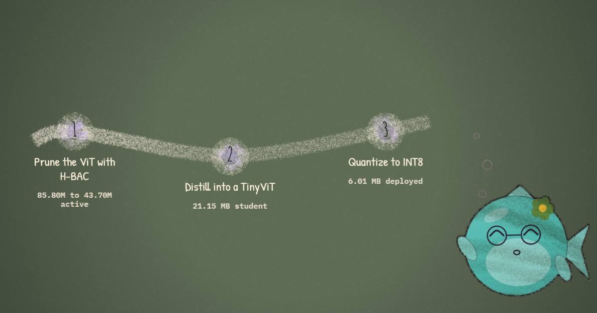
The paper (Kumar, Gondi, Swapnith, Jogi, Manalil, Raha, Mukherjee, Seethapathy & Gopakumar, arXiv 2609.05334) compresses a ViT-B/16 leaf-disease classifier from 327 MB to 6 MB using three techniques at once: a Hessian-guided pruning method the authors call H-BAC, attention-based knowledge distillation, and INT8 quantization. What makes it worth a close read isn't the crop or the compression ratio — it's that the paper explicitly frames its own contribution as answering a question the compression literature mostly ducks: pruning, quantization, and distillation are almost always evaluated in isolation, so does chaining them actually compound their gains, or do the gains overlap? The paper says outright that "the potential benefits and interactions of their combined application" are "insufficiently explored" in prior work. That's a checkable claim against the paper's own ablation tables, and this piece checks it.
| Paper | arXiv 2609.05334 · HTML · PDF |
| Subject | Chilli (Capsicum annuum) leaf-disease classification — 3 classes, ViT-B/16 backbone |
| Methods | H-BAC (Hessian-Balanced Adaptive Block Pruning) → Attention-Based Knowledge Distillation → PTQ-Dynamic INT8, chained sequentially |
| Headline | 327.42 MB → 6.01 MB (54.5×), 95.13 ± 2.32% accuracy across 4 runs — statistically level with the FP32 baseline |
| Dataset | 22,829 field images across 4 physically distinct villages; the OOD test split also switches capture device |
| Latency hardware | Apple M4 Pro CPU (Core ML) + a rented NVIDIA RTX 4060 GPU — not the ARM/Android hardware the paper's own motivation names |
| Code / data | No code release found; the dataset is public via Figshare |
A dataset that actually tries to test generalization
Before the compression story, the dataset deserves credit, because it's unusually careful for a crop-disease paper. Three classes — Healthy, Initial ChiLCV (chilli leaf curl virus), Severe ChiLCV — collected on-site at smallholder farms in Coimbatore, Tamil Nadu between June and November 2024. The thing that makes it a real generalization test rather than a random 80/20 split: every split comes from a physically distinct village, and the out-of-distribution split — the one every accuracy number in the paper is actually measured on — additionally switches the capture device.
| Split | Village(s) | Images | Notes |
|---|---|---|---|
| Train | Arasampalayam | 17,655 | |
| Validation | Vadasithur | 2,207 | |
| In-distribution test | Myleripalayam | 2,207 | same device population as train |
| Out-of-distribution (OOD) | Kuladupalayam, Andipalayam | 760 | 3 phones never used elsewhere (Realme C2, Redmi Note 12, Samsung Galaxy S23) |
A model can't win on the OOD split by memorizing a village's dirt-background color or a specific phone sensor's white balance, because those don't recur between train and test. That's a genuinely deployment-realistic stress test, and every accuracy number in this piece — like every accuracy number in the paper — is measured on that 760-image OOD split. It's worth flagging the size while crediting the design: 760 images is roughly 3.3% of the full 22,829-image collection, which is a fairly narrow window through which to certify "field-ready." And "field conditions" describes where the images were collected, not where the model was benchmarked — more on that gap further down.
Fine-tuned end-to-end on the Train split, ViT-B/16 lands here:
| Metric | Value |
|---|---|
| OOD accuracy | 95.13% |
| Precision / Recall / F1 (weighted) | 95.55% / 95.13% / 95.10% |
| Model size | 327.42 MB (85.80M params) |
| CPU latency (Apple M4 Pro, Core ML) | 7.18 ± 0.01 ms |
| GPU latency (NVIDIA RTX 4060) | 5.56 ± 0.004 ms |
That's the number every compression result in this piece is measured against. Now the pipeline that gets applied to it:
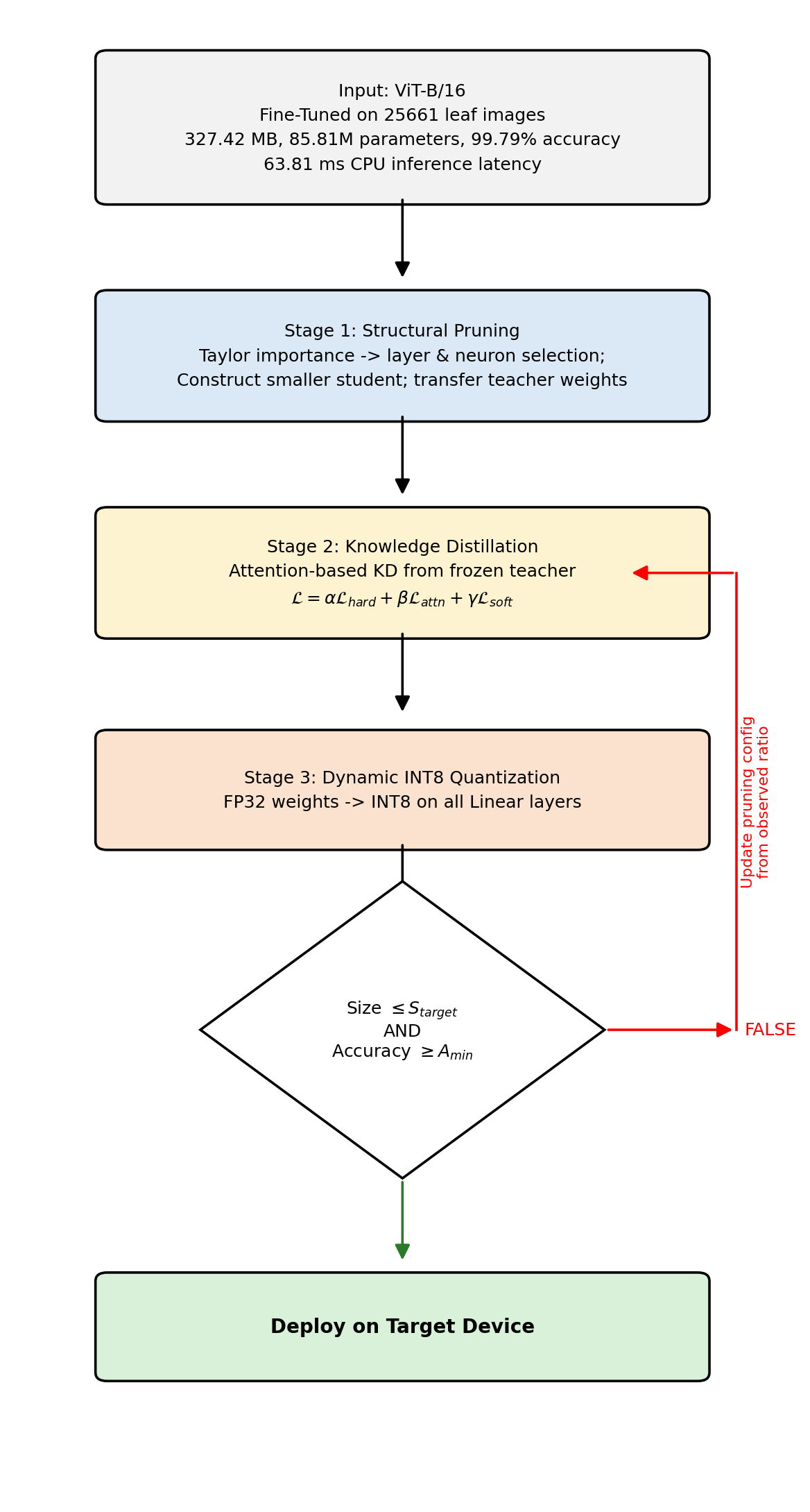
One thing worth flagging about this exact figure: its input box states "25,661 leaf images," "99.79% accuracy," and "63.81 ms CPU inference latency" for the fine-tuned baseline — none of which match the paper's own text or Table 1 (17,655 training images, 95.13% OOD accuracy, 7.18 ms via Core ML). The 63.81 ms figure is plausibly a PyTorch eager-mode CPU number from an earlier pass (the paper notes Core ML is "substantially faster than PyTorch's eager-mode CPU execution" on this hardware), and 99.79% plausibly an in-distribution or training-set figure rather than the OOD number used everywhere else — but the paper doesn't say, and the diagram was never updated to match the numbers its own tables report. It's a small, checkable inconsistency, and a reminder to read a paper's own tables rather than its diagrams when the two disagree.
H-BAC: pruning with a curvature budget, then a first-order scalpel
H-BAC (Hessian-Balanced Adaptive Block Pruning) is a two-level scheme. A second-order signal decides how much to prune each of ViT-B/16's 12 transformer blocks — a budget-allocation problem. A first-order signal then decides which attention heads and MLP neurons to remove within each block, once that block's budget is fixed. That two-level split is the whole design, and it's a real answer to a real problem: the full Hessian of an 85.8M-parameter network is intractable — its memory and compute cost grow quadratically in the parameter count, which is why classical second-order pruning (LeCun's Optimal Brain Damage, Hassibi's Optimal Brain Surgeon) never got applied at transformer scale without heavy approximation.
H-BAC's way around this is the Hutchinson trace estimator: instead of forming the Hessian , it estimates only — a single scalar curvature summary per block — using random probe vectors:
where each is a random Rademacher vector (entries ). can be computed as a Hessian-vector product without ever materializing — the standard double-backprop trick — so the cost per block drops from to , where is the block's parameter count. The paper uses samples per block. This is exactly the trick behind Hessian-Aware Quantization (HAWQ), which uses the same Hutchinson-trace-per-layer signal to allocate bit-width rather than pruning ratio — H-BAC borrows the sensitivity estimator and repurposes it for a different resource. The paper also compares itself directly to NViT, a prior Hessian-based ViT pruner: NViT computes one unified saliency score per weight for global pruning, while H-BAC keeps the second-order signal at block granularity (to stay tractable) and hands off to a separate first-order criterion for the within-block decision.
Attention parameters and MLP parameters are scored separately per block and combined with a balance coefficient (needed because attention and MLP layers differ enough in parameter count and gradient scale that, unweighted, the MLP term would simply dominate):
Block curvatures are then turned into per-block pruning ratios. Note the square root — curvature traces can span orders of magnitude across blocks, and the square root compresses that range before it's turned into a budget:
Given a global pruning target (e.g. 50%), each block's ratio is clipped to , rescaled so the mean across blocks equals again (clipping alone doesn't preserve the mean once curvature is skewed across blocks), then re-clipped, since rescaling can push a ratio back outside the bounds:
Algorithm: H-BAC
Input: pretrained ViT M with B blocks, calibration set D_calib,
       global ratio r, Hutchinson samples K, MLP balance λ

# Phase 1 — block-level curvature (Hutchinson trace, per block)
for b in 1..B:
    for (x, y) in D_calib:
        ℓ = loss(M(x), y)
        H_attn = hutchinson_trace(∇²_attn ℓ, K samples)
        H_mlp  = hutchinson_trace(∇²_mlp  ℓ, K samples)
        c_b += H_attn + λ * H_mlp
    C[b] = max(c_b, 0) / |D_calib|

# Phase 2 — turn curvature into a per-block pruning budget
W = sqrt(C) / mean(sqrt(C))
R = clip(r * W, 0.05, 0.95)
R = r * R / mean(R)              # re-center to the global target
R = clip(R, 0.05, 0.95)          # re-clip after rescaling

# Phase 3 — first-order Taylor pruning within each block's budget
for b in 1..B:
    score attention heads by  I_j = mean_batch⟨∂ℓ/∂f_j, f_j⟩
    zero the ⌈R_b · H⌉ lowest-scoring heads' Q/K/V + output slices
    score MLP neurons by      I_n = |∂ℓ/∂w_n ⊙ w_n|
    zero the ⌈R_b · N⌉ lowest-scoring neurons' fc1 rows / fc2 columns

# Phase 4 — recovery fine-tuning (masks act as gradient masks)
fine-tune M' for 1 epoch, unfrozen, reduced learning rate
The within-block criteria are both classic first-order saliency: attention heads are scored by a Taylor-expansion importance (gradient · activation, Frobenius inner product), MLP neurons by gradient · weight magnitude — the same family of cheap, per-parameter signals that has been standard since magnitude- and Taylor-based pruning entered the literature, applied here only after the expensive second-order signal has already decided each block's budget.
The one genuinely surprising result in this section: pruning ratio should, in the textbook intuition behind Optimal Brain Damage and most Hessian-based pruning heuristics, protect high-curvature blocks — a block sitting in a sharp region of the loss landscape is the one you'd expect a small perturbation to hurt most. H-BAC does the opposite: higher curvature gets pruned more, not less. The paper tested both directions at a 50% global ratio, and the "wrong" direction empirically wins by a wide margin:
| Weighting | Pre-finetune acc. | Post-finetune acc. |
|---|---|---|
| Uniform (no curvature signal) | 41.32% | 93.16% |
| Inverse (protect high-curvature blocks — the textbook intuition) | 34.21% | 94.21% |
| Direct (prune high-curvature blocks more — what H-BAC actually uses) | 64.87% | 95.53% |
Direct weighting beats uniform pruning by 23.55 points pre-finetune and 2.37 points post-finetune; the "theoretically motivated" inverse variant does worse than even the uniform baseline pre-finetune. The paper confirms this empirically and states plainly that it runs counter to the inverse-curvature intuition in the literature — but it doesn't offer a mechanism for why. One informed guess, offered here and not in the paper: block-level curvature under this Hutchinson estimate may be tracking something closer to "how quickly this block's loss surface bends" than "how fragile this block's function is" — and a block that bends fast is also a block that a single epoch of recovery fine-tuning can reshape fast. That's speculation, not a claim the paper makes; it's flagged as such because the result is real and the explanation isn't given.
Sweeping the global pruning ratio from 10% to 90% (Table 5 in full) shows the same pattern holding at every ratio tested:
| Ratio | Active params (M) | FLOPs (G) | Pre-FT acc. | Post-FT acc. | CPU (ms) | GPU (ms) |
|---|---|---|---|---|---|---|
| 0 (baseline) | 85.80 | 35.13 | 95.13% | 93.95% | 7.13 | 5.560 |
| 10% | 77.14 | 31.57 | 94.87% | 96.45% | 6.76 | 5.034 |
| 20% | 68.56 | 28.04 | 89.34% | 96.32% | 6.13 | 4.554 |
| 30% | 60.34 | 24.68 | 73.03% | 94.61% | 5.50 | 4.027 |
| 40% | 51.72 | 21.13 | 68.68% | 97.37% | 4.88 | 3.494 |
| 50% | 43.70 | 17.86 | 64.87% | 95.53% | 4.27 | 3.003 |
| 60% | 36.30 | 14.81 | 53.42% | 94.08% | 3.62 | 2.489 |
| 70% | 29.37 | 11.98 | 34.21% | 91.97% | 3.27 | 2.138 |
| 80% | 25.75 | 10.50 | 33.03% | 93.68% | 2.96 | 1.888 |
| 90% | 22.88 | 9.32 | 34.21% | 91.84% | 2.62 | 1.649 |
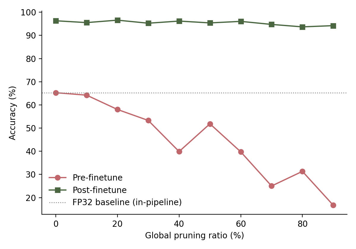
Pre-finetune accuracy collapses steadily toward chance as pruning gets more aggressive — exactly what you'd expect from stripping function with no recovery step. Post-finetune, the story is flat: accuracy stays in a 91.84–97.37% band across the entire sweep, with 90% pruning (91.84%) sitting within two points of the gentlest ratios tested. One epoch of recovery fine-tuning does almost all the work of absorbing pruning damage on this dataset, at any ratio the paper tried. That's a genuinely useful practical finding — it means the pruning ratio's main lever, once recovery fine-tuning is in the pipeline (which it always is here), is FLOPs and active-parameter count, not final accuracy. It's also a reason to treat the single-run 50% number with some caution: if the curve is this flat and somewhat noisy run to run (see the knowledge-distillation variance below), a single point estimate at any one ratio is not a tight bound on what that ratio "really" gets you.
Quantization: real size savings, no measured speed
Two post-training INT8 variants, both applied directly to the trained FP32 checkpoint with no extra fine-tuning:
| Method | Size | Acc. | Δ Acc. | CPU latency | Speedup |
|---|---|---|---|---|---|
| FP32 baseline | 327.42 MB | 95.13% | — | 7.18 ms | 1.00× |
| PTQ-Dynamic | 84.42 MB | 94.34% | −0.79 | 7.21 ms | 1.00× |
| PTQ-Static | 85.78 MB | 94.61% | −0.52 | 7.21 ms | 1.00× |
Both variants land around a 74% size reduction — expected, since INT8 is roughly a quarter the storage cost of FP32 on the Linear layers being targeted. PTQ-Static's 0.27-point edge over PTQ-Dynamic is inside normal run-to-run noise; the paper adopts PTQ-Dynamic throughout for its simplicity (no calibration set required). The number worth sitting with is the speedup column: 1.00×, for both. On this Apple M4 Pro / Core ML setup, INT8 quantization buys none of the inference-time speedup that INT8 usually advertises, because Core ML's weight-only INT8 path dequantizes weights back to floating point before the matmul rather than running native INT8 arithmetic — so the per-operation cost is essentially unchanged. Quantization's entire measured benefit here is file size, not latency. That's a hardware- and runtime-specific fact, not a property of INT8 in general, but it's exactly the kind of thing a compression paper can only tell you by actually measuring on a target runtime instead of assuming the textbook speedup transfers.
Knowledge distillation: three variants, a 0.53-point spread
The teacher (ViT-B/16, 327.42 MB, 85.80M params) distills into a TinyViT student (21.15 MB, 5.52M params, ImageNet-21k pretrained) — a 15.48× compression ratio by architecture swap alone, before any quantization. Three distillation signals were compared against a no-distillation control (mean ± std over 3 runs):
Response-based distills soft-label agreement. Temperature-scaled softmax on both teacher and student logits (), combined with the hard-label cross-entropy:
Feature-based matches intermediate representations at layers 11. Since the teacher's hidden dimension (768) doesn't match the student's (192), a learnable 2-layer MLP adapter bridges the gap before the MSE:
Attention-based skips the dimension-mismatch problem entirely by matching attention maps instead of raw features — a matrix of pairwise patch relationships is dimension-agnostic, so no adapter is needed. Teacher (12 heads) and student (3 heads) attention are each averaged across heads at the same four layers before the comparison:
with the same as feature KD. The pitch, stated plainly by the paper: attention maps encode which patches a model relates to which — e.g. a diseased region attending to healthy tissue for contrast — so this transfers reasoning, not raw activations, and does it without ever needing an adapter network.
| Method | Size | Compression | Accuracy | CPU speedup |
|---|---|---|---|---|
| Teacher (ViT-B/16) | 327.42 MB | 1.00× | 95.13% | 1.00× |
| No distillation (labels only) | 21.15 MB | 15.48× | 96.58 ± 0.26% | 7.07× |
| Response KD | 21.15 MB | 15.48× | 96.27 ± 0.65% | 7.07× |
| Feature KD | 21.15 MB | 15.48× | 96.18 ± 0.60% | 7.07× |
| Attention KD | 21.15 MB | 15.48× | 96.71 ± 1.03% | 7.07× |
All four recipes cluster inside a 0.53-point band. Attention KD wins on mean accuracy, narrowly, and is the only variant to beat the no-distillation control at all — but it also carries the widest run-to-run spread of the four (±1.03 vs. ±0.26 for the control), so "the best distillation method" and "the method whose single run you'd get" are not quite the same claim. The honest read the paper offers itself: distillation's benefit over plain label-training is real but modest on this task, and shouldn't be assumed a priori for a new deployment target.
A follow-up capacity sweep pushes below TinyViT's 5.52M parameters, training four smaller architectures from scratch (no pretrained checkpoint exists at these sizes) with and without Attention KD, 3 runs each:
| Params | No-KD | Attention KD | Advantage |
|---|---|---|---|
| 1.31M | 77.24 ± 13.75% | 70.26 ± 19.15% | −6.97 ± 32.59 pp |
| 1.89M | 70.57 ± 19.35% | 76.80 ± 15.86% | +6.23 ± 34.25 pp |
| 2.63M | 77.15 ± 6.01% | 81.32 ± 8.92% | +4.17 ± 5.41 pp |
| 3.16M | 90.35 ± 0.88% | 82.11 ± 8.07% | −8.25 ± 8.07 pp |
Run-to-run variance dominates completely here — standard deviations of 15–35 points on a "3-run mean," with the advantage's own confidence interval spanning both signs at every size except 2.63M. Training small, non-pretrained ViT variants from scratch on ~17K images is evidently a much less stable process than fine-tuning a pretrained backbone, and this table is the clearest evidence in the paper that single-run point estimates elsewhere in this piece — including the traced 50%-pruning pipeline run below — need to be read with that instability in mind, even where the paper doesn't report a std for them directly.
Does chaining the three actually compound the gains?
This is the question the paper frames as its central contribution, and it's checkable directly against the standalone numbers above. If H-BAC, PTQ-Dynamic, and Attention KD's accuracy effects were independent, you'd add their deltas from the 95.13% baseline: +0.40 (H-BAC) − 0.79 (quantization) + 1.58 (KD) = +1.19 points, predicting a combined pipeline around 96.3%.
The measured pipeline, averaged over 4 runs, lands at 95.13 ± 2.32% — a full 1.19-point shortfall from the naive-additive prediction, and effectively back at the FP32 baseline despite chaining three techniques that all individually helped or cost only a little. The single traced 50%-pruning run (the one Table 4 walks stage by stage) lands at 91.97% — a 4.35-point shortfall from the same prediction. The paper discloses one concrete, measured reason the pieces don't compose cleanly: Attention KD run from the H-BAC-pruned-and-finetuned teacher reaches 93.68%, 1.84 points below the same KD recipe run from the full, unpruned teacher (95.53%) under otherwise identical settings. Pruning first measurably degrades what the teacher has left to distill.
That points straight at the order question. The pipeline runs prune → distill → quantize, and the paper's stated reasoning is procedural: each stage further compresses the model, and quantization has to go last because it's a deployment-precision step applied to whatever weights exist at the end (there's no obvious way to prune or distill through an INT8 checkpoint without extra machinery). What the paper does not do is ablate the prune-vs-distill ordering directly — there's no experiment running distillation before pruning, or quantizing before either. The one order-sensitivity number it does have is the 1.84-point gap above, and that gap arrives as a side effect of comparing two different sections of the paper (the standalone KD ablation vs. the pipeline's KD stage) rather than as a dedicated ordering study. It's real, disclosed, and measured — but it's evidence for a cost of this specific order, not proof that this order was chosen because it was shown to be best among alternatives.
Table 4 walks the traced 50%-pruning run stage by stage:
| Stage | Accuracy | Size | Active params | CPU | GPU |
|---|---|---|---|---|---|
| FP32 baseline | 95.13% | 327.42 MB | 85.80M | 7.18 ms | 5.560 ms |
| H-BAC pruned (pre-finetune) | 64.87% | 327.42 MB | 43.70M | 7.18 ms | 5.560 ms |
| H-BAC pruned (finetuned) | 95.53% | 327.42 MB | 43.70M | 7.18 ms | 5.560 ms |
| + Attention KD | 93.68% | 21.15 MB | 5.52M | 1.02 ms | 0.660 ms |
| + PTQ-Dynamic (deployed) | 91.97% | 6.01 MB | 5.52M | 1.02 ms | — |
| Direct-trained alternative* | 94.87% | 6.01 MB | 5.52M | 1.02 ms | — |
* Skips H-BAC and KD entirely — a fresh TinyViT trained on ground-truth labels only, then quantized with the same PTQ-Dynamic step.
That last row is the paper's most valuable disclosure, and it's worth stating plainly: a model that never saw H-BAC or distillation reaches the identical 6.01 MB footprint at 94.87% accuracy — 2.89 points above the traced pipeline run, and only 0.26 points behind the pipeline's own 4-run mean. One more detail worth a beat: of the four full-pipeline runs the paper reports (91.97%, 97.24%, 96.45%, and 94.87% at a 70% pruning ratio), the last one matches the direct-trained baseline's 94.87% to two decimal places. On a 760-image test set that's less spooky than it sounds — accuracy only takes one of 761 possible values, so exact ties are far more likely than they'd be on a continuous metric — but it's still two differently trained models landing on the same number, which is worth noticing rather than explaining away. The paper's own conclusion, stated in its final section, is that the pipeline's run-to-run variance is the larger effect here, not any consistent accuracy benefit from chaining H-BAC and distillation ahead of quantization. On size alone the three techniques do compound close to multiplicatively — 15.48× from distillation times roughly 3.5× from quantizing the distilled student comes out near the reported 54.5× — though even there it falls about 9% short of naively multiplying distillation's own 15.48× by quantization's own standalone ratio on the full model (3.88×, from 327.42 → 84.42 MB): quantizing the already-distilled student compresses less efficiently (3.52×) than quantizing the full model does, presumably because a larger share of the smaller model's footprint sits in things INT8 doesn't touch. On accuracy, the honest summary is that H-BAC and distillation do real, independently-verified work — but the paper's own numbers don't yet show that chaining them ahead of quantization outperforms simply training a target-sized model directly, at least on this dataset.
Plotted against either size or latency, only two configurations sit on the Pareto frontier at all: Attention KD alone (21.15 MB, 96.71%) and the integrated pipeline's own 4-run mean (6.01 MB, 95.13%) — and the frontier is a coin flip away from being one point, since the pipeline's single traced run (91.97%) is strictly dominated by the direct-trained same-size alternative. The FP32 baseline itself is dominated on both axes by KD alone. On the latency axis specifically, everything the paper measured at the fastest tier (1.02 ms: KD alone, both pipeline variants, and the direct-trained alternative) is beaten on accuracy by plain distillation with nothing else added — the entire 7× CPU speedup in this paper comes from KD's architecture swap to TinyViT, not from pruning or quantization.
The constrained-search mode: a different way to ask the question
Beyond the fixed pipeline above, the paper implements a second mode: given a size budget and an accuracy-drop budget, search for the least aggressive configuration that satisfies both, cascading through 12 candidate stages of increasing aggressiveness (H-BAC alone, H-BAC + quantization, the KD student in FP32, the KD student quantized, then four smaller from-scratch architectures in both precisions). Within the two pruning-ratio families, size and accuracy are both monotone in the ratio, so a bisection search finds the best-fitting ratio in evaluations instead of a linear sweep.
Across 5 size budgets × 2 accuracy-drop budgets (10 combinations), all 10 were satisfiable — but the two loosest and three tightest budgets are met by entirely different mechanisms:
| Size budget | Stage reached | Configuration | Accuracy | Size |
|---|---|---|---|---|
| 25–30 MB | 3 | Plain KD-distilled student (FP32) | 93.68% | 21.15 MB |
| 10–20 MB | 9 | A 1.89M-param student, trained from scratch, no KD | 94.08% | 7.27 MB |
At the tightest budgets, the search abandons the fixed pipeline's own architecture family entirely and jumps to a smaller from-scratch student the H-BAC+KD pipeline never considers — because the KD student quantized to 6.01 MB comfortably meets the size target but blows the accuracy-drop budget (a 3.16-point drop against even the loosest 3% budget tested). A search restricted to the fixed pipeline's own stages would have reported no feasible model under 21 MB at all, despite one existing. That's a genuine demonstration of the constrained-search mode's value over the fixed pipeline — and also, again, a case where the simplest available baseline (train small, don't distill) wins.
What "on-device" means here, and what it doesn't yet
Every latency number in this piece — 7.18 ms baseline CPU, 1.02 ms distilled CPU, the whole GPU column — was measured on an Apple M4 Pro laptop CPU (via Core ML) and a rented NVIDIA RTX 4060. Neither is the hardware this paper's own introduction motivates: "low-end mobile devices that represent the primary computing resource available to most rural farmers." The paper says this itself, directly and near its conclusion, without hedging: these devices "were chosen because they give controlled, reproducible measurements suitable for comparing compression techniques against each other," the size and FLOPs reductions are device-independent and are what the deployment argument actually rests on, and "the absolute latency numbers... should not be read as predictions of on-device farmer-facing performance." Validating on actual ARM smartphone-class hardware (Snapdragon or MediaTek, via TensorFlow Lite, ONNX Runtime Mobile, or Core ML conversion) is named explicitly as future work.
So: is this a compression paper about FLOPs, or a paper with a measured deployment target? By the paper's own account, it's the former, honestly labeled. The size reductions (74–98%) and the FLOPs reduction from pruning (49%) are real and hardware-independent claims. The latency numbers are real measurements, but of a laptop CPU and a cloud GPU standing in for a phone that was never benchmarked. And the one latency number that would most directly inform "does INT8 help on the target class of hardware" — quantization's speedup — came back at 1.00× on the hardware actually used, for a runtime-specific reason (Core ML's weight-only INT8 dequantizes to float before the matmul) that may or may not hold on an ARM NPU or a mobile GPU delegate. Every one of these caveats is disclosed in the paper's own text; none of them is hidden. What's missing is simply the measurement that would resolve them.
The honest read
Take this paper on its own terms and it holds up better than its abstract's headline compression ratio alone would suggest. The dataset design — cross-village, cross-device OOD evaluation — is genuinely more rigorous than a random split, and the paper is unusually willing to publish results that complicate its own pitch: the direct-trained same-size baseline, the sub-additive pipeline math, the inverse-curvature result that contradicts textbook intuition and gets reported anyway, the explicit "this isn't the target hardware" caveat. H-BAC's Hutchinson-trace curvature signal is a real, tractable second-order sensitivity estimate rather than a first-order stand-in wearing a second-order name, and the direct-vs-inverse weighting result is a genuinely interesting, currently unexplained finding that someone should dig into.
What isn't yet shown: that chaining pruning, distillation, and quantization outperforms the much simpler alternative of training a target-sized model directly, on this dataset, at this operating point. The four reported pipeline runs (91.97%, 94.87%, 96.45%, 97.24%) span a 5.27-point range around a 95.13% mean — a band wide enough that the 94.87% direct-trained baseline sits inside it, exactly matches one run, beats a second, and loses to the remaining two. A single crop, three classes, a 760-image OOD test set, and latency measured on hardware nobody will actually run this model on are all real scope limits the paper names itself. None of that makes the work uninteresting — it makes it an unusually honest ablation study about when compression composability holds and when it doesn't, on one real, if narrow, agricultural deployment problem.
For more on the pieces this paper leans on: how self-attention actually works underlies both the attention-map distillation signal and H-BAC's per-block attention curvature term; Nemotron's NVFP4 covers a very different point on the quantization spectrum (training natively in 4-bit rather than post-training INT8); and MimiModel is the same "real deployment target, real honesty about the numbers" spirit taken to its extreme — a 45M model on a $5 microcontroller chip.