2026-10-08 · 25 min · quantization · on-device · distillation · kernels · kv-cache
Why read this
Notabletop 60%Does LittleBit's 0.1-bit arithmetic on real Llama2 shapes, re-runs its initialization on real weights, and checks which comparisons are QAT against PTQ.
- Original analysis
- A lasting reference
- A new technique
Quantization & compressionNeeds datacenter GPUsNon-commercial licenceResearch paper
How this was scored
- Is it new?
- 2 of 3: A real new idea, method or capability
- Can I trust it?
- 2 of 3: Measures key facts from files, code or configs
- Can I run it?
- 1 of 3: API-only, gated or restrictive licence
- Will I understand it?
- 2 of 3: Mechanism from first principles with figures
- Can I act on it?
- 2 of 3: A concrete recipe, numbers or comparison
- Will it last?
- 2 of 3: A reference for a year or more
- Does it affect many?
- 1 of 3: A specialist community
- Only here?
- 2 of 3: A teardown or measurement few others did
Score 62 of 100, ranked 217 of 476 rated articles. Each question is answered 0–3 by hand, and a 3 is rare. How articles are scored
"0.1 bits per weight" is a strange number, and that is why I opened the paper. A bit is the smallest thing you can store. A tenth of one per weight means one stored bit for every ten weights of the original model, and no weight anywhere gets a bit of its own. The abstract says this puts Llama2-13B "under 0.9 GB" and that LittleBit at 0.1 BPW "surpasses the performance of leading techniques operating at 0.7 BPW on Llama2-7B".
The paper is LittleBit: Ultra Low-Bit Quantization via Latent
Factorization by Banseok Lee, Dongkyu Kim, Youngcheon You and
Youngmin Kim at Samsung Research, accepted at NeurIPS 2025. I read v5 (5 February 2026) and
compared it against v1 (30 May 2025). The code is at
SamsungLabs/LittleBit, which I cloned at commit
933857e (7 May 2026) and read in full.
- license
- CC-BY-NC-4.0
- branch
- main
- tests
- none found
- source
- 98.1 kB
- commit date
- 2026-05-06
by size of tracked source at this commit, file counts in brackets; docs, data and vendored trees excluded
local clone, 2026-10-08 at 933857e — branch, commit, commitDate, fileCount, hasTests, languages, license, licenseFile, shallow
shallow clone: counts describe the pinned tree, not the history
I wanted three answers. How do you count a tenth of a bit, and is the count honest? What does a model at that rate actually do? And does anything get faster? The short version: the counting is honest and the trick is genuinely clever, the model at 0.1 BPW is a research artefact rather than something you would talk to, and the speed story is real at the kernel level but the kernel is not in the repository.
You can't binarize your way below one bit
Every 1-bit method before this one has the same floor. If each weight becomes a sign, you pay one bit per weight plus whatever the scales cost, so you end up at 1.0 to 1.1 BPW. The Ternary15M model on this site sits at about 1.58 for the same reason: the format is per-weight, so the floor is per-weight too. STBLLM, the previous sub-1-bit method LittleBit compares against, gets under one bit by pruning: N:M structured sparsity throws away whole weights (4:8 for 0.55 BPW, 2:8 for 0.30) and binarizes the rest.
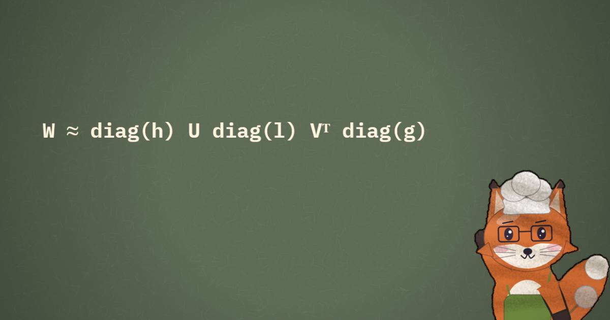
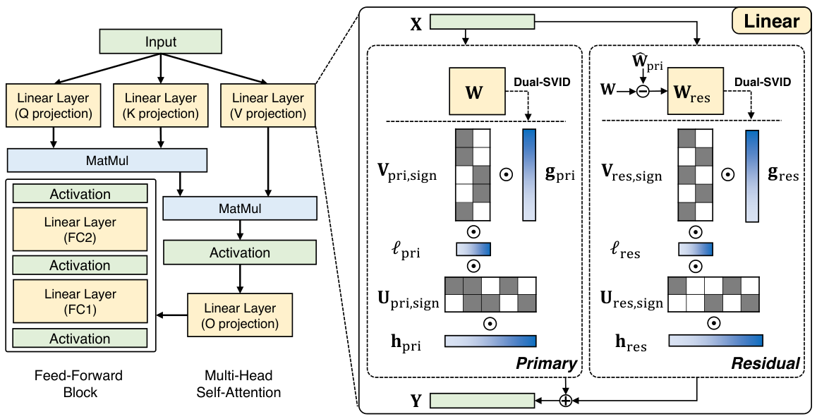
LittleBit gets under the floor a different way: it stops storing weights at all. A linear layer is first written as a low-rank product with and . Then the two factors, not the weight, are binarized. What you store is two sign matrices and three scale vectors, and the paper's Equation 4 rebuilds the effective weight from them:
Here and cost one bit per entry. scales output rows, scales input columns, and is the new piece: a latent scale that says how much each of the rank-one components matters. All three are FP16. Row and column scales are standard in 1-bit work; OneBit uses them. The latent scale exists because the factorization creates a third axis that the other two can't see.
The storage is now proportional to rather than . Pick small enough and the sign bits, divided by the number of original weights, fall below one.
Counting a tenth of a bit
Appendix D gives the count, and quantization/modules/littlebit.py:88-97 implements the same
formula. With the residual path (more on it below) a layer has two copies of everything:
The first term is the sign bits, the second the two pairs of and
vectors at 16 bits each, the third the two vectors. You solve it for
given a target . The code does that at littlebit.py:55-67, then floors the result to a
multiple of 8 (littlebit.py:80-81), so the realized rate always lands a little under the
target.
Take a real shape. Llama2-7B's q_proj is 4,096 x 4,096, which is 16,777,216 weights. At a
0.1 target the formula gives 86.2, and the code floors it to per path. Then:
- sign bits:
- scale bits:
- total: 1,575,424 bits, or 0.0939 bits per original weight
The MLP's down_proj is 4,096 x 11,008, 45,090,816 weights. The paper's worked example lands on
; the code's floor gives 128. That is 3,866,624 sign bits plus 487,424 scale bits,
0.0966 BPW.
Two things fall out of this that the paper doesn't dwell on. First, the FP16 scales are not
free at this rate: they are 16.8% of the q_proj budget and 11.2% of the down_proj budget.
Second, each path is a rank-80 sign matrix pair for a 4,096-wide layer. The model is
expressing a 4,096 x 4,096 projection with 80 binary directions, twice. The calculator below
does this for every layer of Llama2-7B, 13B and 70B, with the code's rank rule.
| layer | d_out x d_in | rank r | sign bits | scale bits | bits/weight |
|---|---|---|---|---|---|
| q_proj | 4,096 x 4,096 | 2 x 80 | 1,310,720 | 264,704 | 0.0939 |
| k_proj | 4,096 x 4,096 | 2 x 80 | 1,310,720 | 264,704 | 0.0939 |
| v_proj | 4,096 x 4,096 | 2 x 80 | 1,310,720 | 264,704 | 0.0939 |
| o_proj | 4,096 x 4,096 | 2 x 80 | 1,310,720 | 264,704 | 0.0939 |
| gate_proj | 11,008 x 4,096 | 2 x 128 | 3,866,624 | 487,424 | 0.0966 |
| up_proj | 11,008 x 4,096 | 2 x 128 | 3,866,624 | 487,424 | 0.0966 |
| down_proj | 4,096 x 11,008 | 2 x 128 | 3,866,624 | 487,424 | 0.0966 |
q_proj: two paths of rank 80. Signs are 1,310,720 bits, the FP16 scale vectors 264,704 (16.8% of the layer), against 16,777,216 original weights: 0.0939 bits each on disk, 1.27 once the released loader has unpacked the signs into bf16.
The linear layers drop from 13.0 GB to 0.077 GB (167x). The whole model drops from 13.5 GB to 0.602 GB (22.4x), because the embedding and lm_head stay in FP16 and are 87% of what is left.
The calculator's last toggle is the one I care about most, and I'll come back to it under
inference. The one to look at first is the size bar. At 0.1 BPW the 6.48 billion
linear-layer weights of Llama2-7B fit in 77.5 MB. The token embedding and the lm_head stay in
FP16, as the paper says in its Table 3 caption and the code enforces
(quant_util.py:166, exclude_names=["lm_head"]; the embedding is an nn.Embedding, not an
nn.Linear, so the patcher never touches it). Those two matrices are 32,000 x 4,096 each,
524 MB together. My total is 0.602 GB, of which 87% is the part LittleBit doesn't compress.
The paper's Table 3 says 0.63 GB; I get numbers a few percent below theirs at every rate and
couldn't pin down the difference, but it doesn't change the picture.
So "Llama2-13B under 0.9 GB" is true (Table 3 says 0.84 GB, 31.02x) and also mostly a statement about the embedding: of my 0.81 GB for 13B, 81% is the 655 MB of FP16 embedding and lm_head. The transformer blocks themselves shrink by about 167x on 7B. The paper acknowledges the embedding bottleneck in its Limitations section (Appendix I), and I don't think it is a flaw in the method. It does mean the headline ratio is set by a component the method leaves alone, and that 0.1 BPW on the blocks buys you very little over 0.3 in whole-file terms: 0.60 GB against 0.76 GB on 7B.
Starting from signs: Dual-SVID
You can't train a rank-80 binary factorization from random signs and expect it to find
Llama2's q_proj. The paper says naive initialization makes QAT unstable, and its fix is the
part of the method I like best.
Start from the truncated SVD, , with the
singular values split evenly between the factors (the code does
U = U_t @ sqrt(S), V = sqrt(S) @ Vh at littlebit.py:287-290). Now separate each factor
into what binarization keeps and what it throws away. The sign is kept exactly:
. The magnitude is a
nonnegative matrix, and the method approximates it by its best
rank-1 factorization, . That
rank-1 factorization is exactly a row scale times a column scale. Do the same for
, and multiply the two latent
pieces: .
The name is literal. "Sign-Value-Independent Decomposition" splits a matrix into a sign pattern and a magnitude, then models the magnitude separately. OneBit introduced SVID on the weight matrix itself. LittleBit does it twice, once per factor, which is where "Dual" comes from, and the structure of the result matches the structure of the layer exactly: the rank-1 pieces become , and with nothing left over. The latent factors , themselves are initialized to , and kept in full precision during training; only their signs are used in the forward pass.
Why is this a good starting point? Because a nonnegative matrix's top singular vectors are nonnegative, so the rank-1 magnitude model never fights the sign pattern, and because SVD factors have a strong per-column magnitude structure (column carries ), which is exactly what is there to capture.
I wanted to see how close this gets in practice, so I re-implemented Dual-SVID in numpy,
following Equations 6-8 and the code line for line, and ran it on three real Llama2-7B
matrices pulled by HTTP range request from the safetensors shards: layer 0's q_proj (the
same tensor as the paper's Figure 3), layer 15's q_proj, and layer 15's down_proj. For each
target rate I used the code's rank rule and measured the relative Frobenius error
.
At 0.1 BPW on layer 15 q_proj (flat spectrum: the top 184 directions hold 36% of the energy): one path gets rank 184, two paths get 80 each. Relative error is 0.798 for the unbinarized SVD, 0.930 for one Dual-SVID path (0.932 without the latent scale) and 0.929 with the residual path. Lower is better; 1.0 means the reconstruction explains nothing.
Three things surprised me.
The starting point is far from the weight. On layer 15's q_proj at 0.1 BPW, Dual-SVID
with both paths has a relative error of 0.929; the reconstruction points in roughly the
right direction (cosine 0.37) but explains little of the matrix. Even the unbinarized
truncated SVD at rank 184 has error 0.798 there, because a mid-layer projection's spectrum
is flat: the top 184 directions hold 36% of its energy. Layer 0's q_proj is the exception,
almost low-rank already (the top 80 directions hold 90% of its energy), which makes it a
flattering choice for a figure.
Error barely moves with rank once you binarize. On layer 0, one Dual-SVID path sits at 0.82 to 0.84 from 0.1 BPW all the way to 1.0, while the unbinarized SVD drops from 0.21 to 0.014. Binarization, not rank, is the bottleneck. The paper predicts this in Appendix A (its Claim 1 says the error "might be non-decreasing with "), and it holds on real weights.
The latent scale earns its place. On layer 0 at 0.1 BPW, setting to a constant takes the error from 0.823 to 0.910; at 1.0 BPW, from 0.842 to 0.980. On layer 15 it matters much less (0.930 against 0.932 at 0.1 BPW).
There is one more line in the widget worth a look: plain with a rank-1 magnitude, OneBit's initialization, which costs about one bit per weight. On all three matrices it starts closer to (0.603 to 0.627) than LittleBit's two-path initialization does at 1.0 BPW (0.714 to 0.751). I can't prove the two are connected, but it is consistent with LittleBit losing to OneBit at 1.0 BPW in the trained results below: at one bit, binarizing the weight directly keeps more than binarizing a factorization of it.
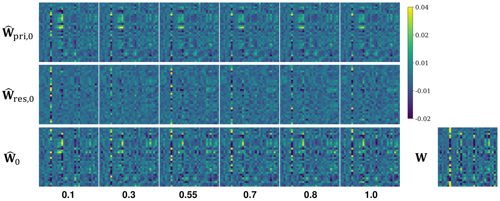
What this tells me is that Dual-SVID's job is not to approximate . It is to put the signs and scales somewhere sensible so that distillation can do the rest. The paper is honest about this in its framing ("a starting point"); the figure it shows makes it look better than it is.
The residual path: same bits, split in two
Residual Compensation sounds like it adds capacity. It doesn't: it spends the same budget
differently. Instead of one path at rank , you get two paths at roughly each, the
second initialized by running Dual-SVID on the error the first leaves behind,
(littlebit.py:197-219). After initialization both paths train jointly, so "residual" only
describes how they start.
What does the split cost? The second path brings its own and , and
those are paid out of the rank. For q_proj at 0.1 BPW, one path gets ; two paths
get latent directions in total. You give up 24 binary directions, 13% of
them, to buy a second set of scales and a second chance at the sign pattern.
At initialization it is worth it on the low-rank layer: on layer 0, the error falls from 0.823
(one path, rank 184) to 0.719 (two paths of 80). That agrees with the paper's Figure 3 claim
that the summed 0.3 BPW initialization beats the primary path alone at 1.0 BPW (0.699 against
0.837 in my run). On the mid-layer matrices at 0.1 BPW the two are a wash: 0.929 against 0.930 on layer 15's
q_proj, and on its down_proj the single path is marginally better, 0.957 against 0.959.
After training, the paper's own ablation is mixed. Table 5 runs OPT-1.3B with and without the residual path: it helps by 1.3 to 1.4 perplexity points from 0.55 to 1.0 BPW, by 0.74 at 0.3, and at 0.1 BPW it hurts badly, 60.011 with the residual against 48.512 without. The authors say larger models "generally showed" a benefit and adopt it everywhere. That may well be true, but the larger-model runs aren't in the paper, and the one ablation that is shown says the residual path is wrong at exactly the rate in the title, at least for a 1.3B model.
How it is trained, and on what
LittleBit is quantization-aware training with knowledge distillation. The FP16 model is the
teacher. The loss is KL divergence on the output logits plus ten times the mean squared error
between every pair of teacher and student hidden states, which is easy to read in
utils/kd_utils.py:46-54:
# utils/kd_utils.py:46-54
kd_loss = self.ce_loss(student_logits, teacher_logits)

l2l_loss = 0
for student_rep, teacher_rep in zip(student_reps, teacher_reps):
    tmp_loss = self.mse_loss(student_rep, teacher_rep)
    l2l_loss += tmp_loss
l2l_loss = self.l2l_loss_scale * l2l_loss

loss = kd_loss + l2l_loss
The sign function has no useful gradient, so the backward pass uses the derivative of
, which the paper calls SmoothSign (quantization/functions/binary.py:20-34).
It beats the straight-through estimator in Table 6, but by little: 60.011 against 60.401
perplexity at 0.1 BPW on OPT-1.3B, and the two are within 0.1 everywhere else. I'd treat it as
a detail, not a contribution.
The data is one C4 shard (en/c4-train.00000-of-01024.json.gz) concatenated with
WikiText-2's training split (utils/datautils.py:259-302). Appendix G says (in a sentence v1 didn't
have) that it is about 1 billion tokens over 5 epochs, roughly 0.2 billion per epoch, on four H100s for
every model except QwQ-32B, which took 32 A100s. The learning rate was swept between 4.0e-5
and 2.4e-4 for every model and every BPW, picking the one that minimized validation
perplexity. There is no wall-clock figure anywhere. The authors also say in Appendix I that
they couldn't run QAT on 70B-class models with their resources, which is why Llama2-70B
appears in the memory table but not the perplexity table.
So this is not post-training quantization. It is a billion-token distillation run per model
per rate, with a per-run learning-rate sweep, on a training mix that contains WikiText-2 and
is evaluated on WikiText-2. The code evaluates on the WikiText-2 test split
(datautils.py:343-352); the paper says "validation". Either way the training text and the
evaluation text come from the same corpus, which favours the trained method on exactly the
metric the headline uses.
Checking the headline against the tables
The paper draws its main result for Llama2-13B.
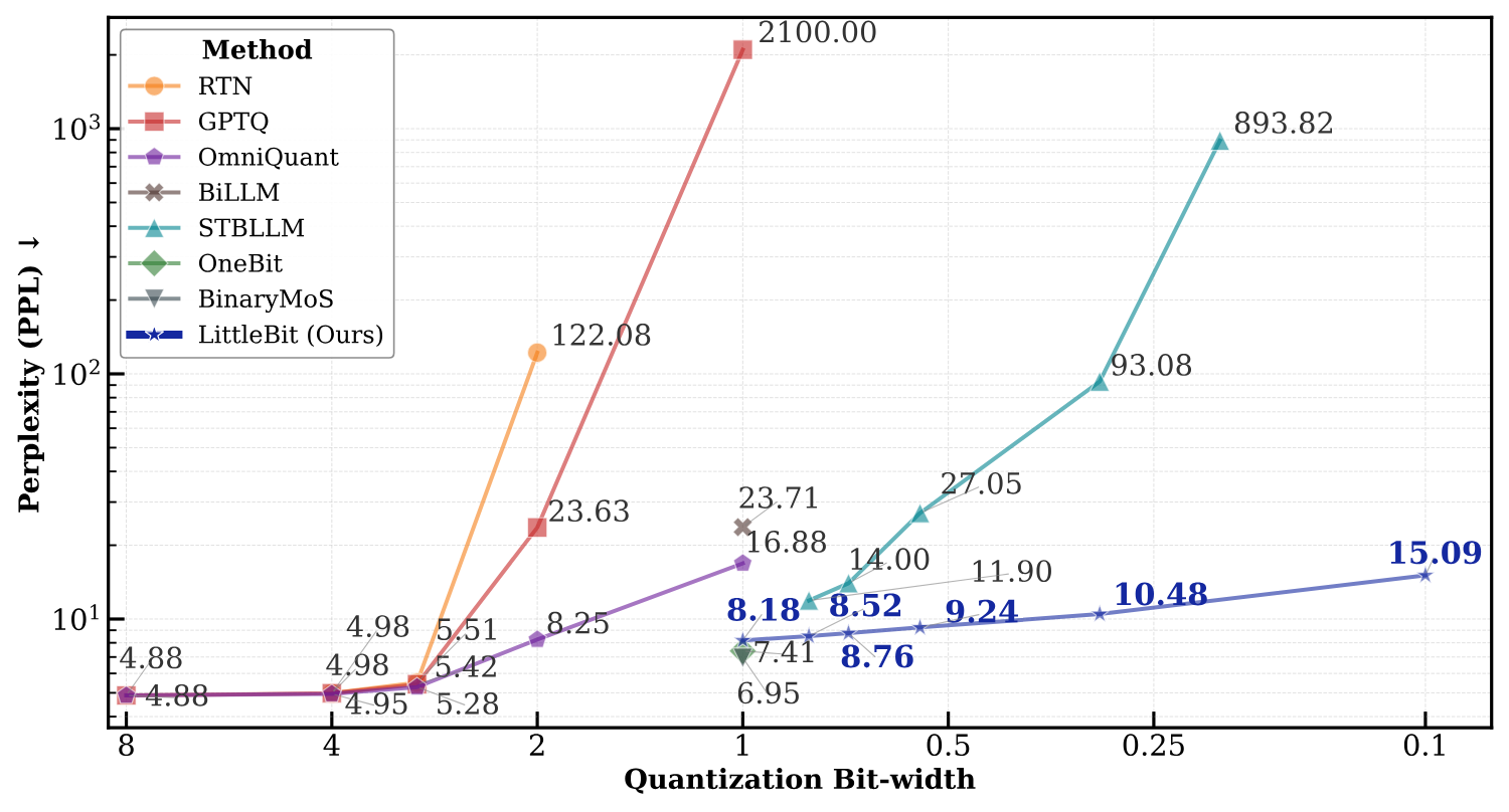
The abstract's comparison is Table 1's Llama2-7B column: LittleBit at 0.1 BPW scores 15.92, STBLLM at 0.7 BPW (5:8 sparsity) scores 19.17. That is accurate. It is also a quantization-aware method with a billion tokens of distillation against a post-training method. The paper's own Baselines paragraph calls STBLLM "a post-training quantization (PTQ) method", and the table marks QAT rows with a dagger; the abstract and introduction don't say it. STBLLM at 0.8 BPW (13.81) still beats LittleBit at 0.1.
The fair comparison is against the other QAT methods, and the paper only has them at 1.0 BPW. There LittleBit loses in every column. On Llama2-7B it scores 9.08 against OneBit's 8.36 and BinaryMoS's 7.74. On QwQ-32B it is 12.08 against 9.86 and 8.99. The paper attributes the BinaryMoS gap to dynamic scaling, which is fair; it doesn't explain the OneBit gap. What LittleBit has that those methods don't is a dial: OneBit can't go below one bit, and LittleBit degrades gently all the way down, and I think that dial is the real contribution.
While matching Figure 1 to Table 1 I found one inconsistency. Table 1 gives STBLLM on Llama2-13B at 0.30 BPW a perplexity of 893.82. Figure 1 plots a point labelled 93.08 at about 0.3 and puts 893.82 further right, at about 0.2 BPW, a setting Table 1 doesn't have. One of the two is wrong. It doesn't change the conclusion, since LittleBit's 10.48 at 0.3 beats either.
How good is 0.1 BPW?
Perplexity first. At 0.1 BPW, Llama2-7B goes from 5.47 to 15.92, about 2.9x FP16. Llama2-13B goes from 4.88 to 15.09, Llama3-8B from 6.10 to 26.11, QwQ-32B from 6.34 to 35.26. At 0.55 BPW, Llama2-7B is 10.47, about 1.9x. The paper itself says "a quantization cliff appears between 0.3 and 0.1 BPW" and names 0.3-0.55 as the sweet spot, which I agree with.
The zero-shot table (Table 2) only goes down to 0.3 for the Llama models, and it needs one correction to read: the chance level. WinoGrande and PIQA are two-way choices (50%), OBQA, HellaSwag and both ARC sets are four-way (25%), and BoolQ's majority class is about 62%. Averaged over the seven tasks, guessing scores about 37.5. Llama2-7B FP16 averages 62.97; LittleBit at 0.3 BPW averages 45.20. Of the 25.5 points FP16 has above chance, 0.3 BPW keeps about 30%. Look at the columns and three of seven are at chance: WinoGrande 51.30, ARC-c 25.09, and BoolQ 61.80, just under the majority class. At 0.55 BPW it keeps about 38%. For Phi-4 at 0.1 BPW the text gives a 43.6% average, which is also not far above chance for that task mix.
The generated samples in Appendix F are the most honest part of the paper. At 0.1 BPW, Phi-4 continues "The Mona Lisa is" into something about a "statue" and "Milan's fashion world", and defines computer science as "the study of the theory and methods of how the human mind and the brain work". The authors' own summary is that the model keeps "superficial grammatical structure" while factual recall collapses. That matches the perplexity: fluent-ish text, little knowledge.
Bytes against bytes
There's a comparison the paper never makes but its own tables allow. If you have a fixed memory budget, should you take a bigger model at fewer bits or a smaller one at more?
At about 0.8 GB: Llama2-13B at 0.1 BPW is 0.84 GB with perplexity 15.09; Llama2-7B at 0.3 BPW is 0.79 GB with 12.00. At about 1 GB: Llama2-7B at 0.55 is 0.98 GB with 10.47; Llama2-13B at 0.3 is 1.15 GB with 10.48. Both times the smaller model at the higher rate is as good or better for less memory. Part of that is the FP16 embedding again (13B's is bigger), but that's the point: the whole file is what you pay for. On these numbers 0.1 BPW is a demonstration that the method degrades gracefully, not the setting you'd pick. And the comparison I'd most want, a small dense model quantized to 4 bits at the same 0.6 GB, isn't in the paper.
Does anything get faster?
The forward pass never builds . Proposition 1 rewrites as a chain of two thin matrix products with element-wise scales in between:
The code is a one-liner at littlebit.py:125, with kept as two vectors
(v1 * u2) that multiply on the fly:
# quantization/modules/littlebit.py:122-125
v1u2 = v1 * u2

# ((((x * v2) @ Vq^T) * (v1 * u2)) @ Uq^T) * u1
return ((((x * v2) @ Vq.t()) * v1u2) @ Uq.t()) * u1
For decoding at batch size 1, the cost of a linear layer is reading its weights from memory. A rank-80 pair of sign matrices is tiny next to a 4,096 x 4,096 FP16 matrix, and multiplying by is a sign flip, not a multiply. Appendix H counts it for a Llama2-7B MLP layer at 0.3 BPW: 90.2 million FLOPs for FP16 against about 13.0 million FLOPs plus 13.0 million bitwise operations for LittleBit.
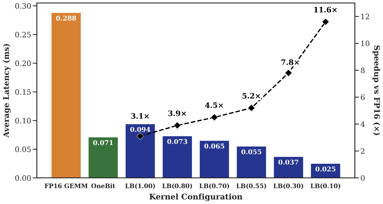
The 11.6x in the abstract is that chart's right-hand bar: one 8,192 x 28,672 layer, batch size
1, 0.2882 ms for torch.matmul in FP16 against 0.0249 ms for the LittleBit kernel at 0.1 BPW.
Table 13 has the rest, and it's more sobering. On the Llama2-7B MLP shape (4,096 x 11,008)
the speedup is 3.23x at 0.55 BPW, 3.23x at 0.3 and 3.26x at 0.1: it stops improving below
0.55 because the layer is now so small that launching kernels and reading activations
dominate. At 1.0 BPW LittleBit's kernel (2.61x) is slower than the OneBit kernel (2.74x).
End to end, with only the linear layers accelerated, Llama2-7B decodes 128 tokens at 203.20
tokens per second against 82.56 for FP16, 2.46x (Table 14).
This part changed the most between versions. In v1 the same 70B MLP benchmark gave 0.053 ms at 0.1 BPW, a 5.42x speedup, and the abstract said "a 5x speedup". By v5 the kernel runs at 0.0249 ms against the same FP16 baseline (0.286 ms then, 0.2882 ms now) and the abstract says 11.6x. The comparison kernel improved just as much: v1's OneBit kernel took 0.257 ms on that layer, v5's takes 0.0713 ms. The end-to-end throughput table is new in v5, as is the training token count. v1's Table 10 also had several Llama2-7B learning rates printed as 4.0e-4 and 8.0e-4 that v5 corrects to 4.0e-5 and 8.0e-5. The perplexity table is identical across the two.
Now the catch. The kernel is not in the repository. I searched every file for CUDA, Triton,
XOR or popcount code and found none. The released forward pass is the PyTorch line above:
Vq and Uq are dense tensors of in the model's dtype, multiplied by ordinary
matmul. And when you load a saved checkpoint, quant_util.py:251-253 unpacks the packed
sign bits back into a dense bf16 tensor (the calculator's third toggle). With it on, a
0.1 BPW Llama2-7B holds 1.34 bits per weight in its linear layers, 1.61 GB for the whole model.
That is still more than 8x smaller than FP16, because the factors are low-rank even when each
sign costs 16 bits. At 0.55 BPW the same loader holds 8.56 bits per weight, 7.46 GB, and the
win over FP16 is under 2x.
The unpacker shifts the wrong way
While reading that loader I tried the pack-unpack round trip by hand. binary_packer stores
sign as bit 1, least significant bit first, 32 signs per int32 word. The unpacker reads
bit of each word like this:
# quantization/utils/binary_packer.py:88
bits = (word_data.unsqueeze(1) << torch.arange(32, device=packed_tensor.device)) & 1
That is a left shift. (w << k) & 1 is zero for every , because shifting left fills
the low bit with zero. Only bit 0 of each word decodes correctly; every other position decodes
as . I re-implemented both functions in numpy (I didn't run the repository's code) and
the round trip recovers 55% of the signs on random input. With >> it recovers all of them.
Since main.py saves through the packing state_dict and eval.py loads through this
unpacker, a model trained and saved with the released code comes back with about half of its
signs flipped to . The paper's numbers can't have come through this path, so I take it
as a regression in the cleaned-up release, not a problem with the results. Someone filed it as
issue #21 on the day I read the code; it
is a one-character fix. There are also no released LittleBit checkpoints that I could find on
Hugging Face, and issue #1 asking for them is still open, so for now the only way to get a
LittleBit model is to train one.
The KV-cache claim
Section 5 says the factorization "inherently compresses the KV cache": if is
computed through a rank- bottleneck, cache the -wide latent instead of the
-wide key, and save , up to 21.3x on Llama2-7B at 0.1
BPW (Table 4, with ). Two problems. The code doesn't do it: Llama attention is
untouched, and the one custom attention module (quantization/modules/attention.py:83-93, for
Phi) applies RoPE to the full keys and caches those. And Llama applies
rotary position embeddings to the key after the projection, so a cached
latent has to be re-expanded through and rotated for every past
token at every step. DeepSeek's MLA, which the paper cites as the analogue, needed a separate
decoupled RoPE key for exactly this reason. The ranks in Table 4 are also close to what the code's rule gives a single path (184 at
0.1 BPW, against the table's 192), while the trained models use two paths of 80. I'd read the KV-cache section as a possibility, not a
result. If KV-cache memory is your problem, TurboQuant attacks
it directly.
What I'd take from it
The idea that will outlive this paper is the change of unit. Binarize the factors of a
low-rank decomposition rather than the weights, and bits per weight becomes a continuous dial
set by the rank instead of a floor set by the format. Dual-SVID is a neat way to make that
dial trainable: it maps an SVD onto exactly the parameters the layer has. Llama2-7B at 0.55
BPW with perplexity 10.47 is a real result, and nothing else in the paper's comparison gets
there. The authors have since extended the initialization: the README describes LittleBit-2
(arXiv 2603.00042, ICML 2026), which rotates the latent
factors toward the binary hypercube before QAT and ships in the same repo behind --use_itq.
I haven't read that paper, so I'll leave its claims alone.
The headline numbers are the weakest part. "0.1 BPW beats 0.7 BPW" is a trained method against an untrained one. At 0.1 BPW the file is mostly embedding, the model is about 2.9x FP16 perplexity with several zero-shot tasks at chance, and a smaller model at 0.3 BPW does better for the same bytes. The 11.6x is one layer shape on a kernel you can't download.
If you're building for a device with a hard memory cap, the honest recipe from this paper is 0.3-0.55 BPW on the transformer blocks, a separate plan for the embedding and lm_head, and four H100s for a billion tokens of distillation per model. The Bonsai 27B release on this site is the opposite trade: a whole network, embeddings included, at 1.125 bits, with kernels that ship. And for what happens when you train in low precision from the start rather than compressing afterwards, see Nemotron in NVFP4.
How I checked
- Paper: read v5 in full from arXiv HTML; the hyperparameter, inference and limitations appendices (G-J) are missing from the HTML build, so I read those in the v5 PDF. I diffed v1's PDF against v5 for the abstract, Table 1, the latency tables and the hyperparameter table.
- Code:
git clone --depth 1of SamsungLabs/LittleBit at933857e; read every Python file. I did not run it. The repository is licensed CC BY-NC 4.0; the paper is CC BY-NC-ND 4.0. - Bit counts and model sizes: computed from the code's rank rule and bit formula for the
Llama2-7B, 13B and 70B shapes in their
config.json(vocabulary 32,000, untied embeddings). The FP16 total for 7B, 13,476,839,424 bytes, matches the safetensors index ofNousResearch/Llama-2-7b-hf. - Dual-SVID: my own numpy re-implementation of Equations 6-8 and
littlebit.py:283-343, run in float64 with exact SVDs onmodel.layers.0.self_attn.q_proj,model.layers.15.self_attn.q_projandmodel.layers.15.mlp.down_proj, read fromNousResearch/Llama-2-7b-hfby HTTP range request. These are initialization errors only; I did not train anything, and they say nothing about the error after QAT. - Unpacker: re-implemented
binary_packerandbinary_unpackerin numpy on a random matrix and checked the round trip with<<and>>. - Chance levels for the zero-shot average: 50% for WinoGrande and PIQA, 25% for OBQA, HellaSwag, ARC-e and ARC-c, and BoolQ's 62% majority class.
- Not checked: any perplexity, zero-shot or latency number in the paper (no checkpoints are released and I didn't train one), and the source of the few-percent gap between my model sizes and Table 3.