PrunaSuperPoint: a 2.1x faster keypoint front-end, pruned where the time actually is

mdjsonmcpcopy↗ai

2026-10-02 · 16 min · pruning · distillation · inference-optimization · on-device · edge-inference · slam · robotics · computer-vision · open-source · explainer

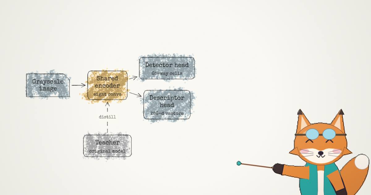
A post from @PrunaAI announced PrunaSuperPoint: an optimized SuperPoint for keypoint detection on edge devices, up to 2.1x faster on a Jetson Orin Nano, built with CEA's Eclipse Aidge for the DeepGreen project, and open. SuperPoint is the model I reach for first when a SLAM front-end needs learned features — the site's SurfSLAM write-up pulls SuperPoint features for place recognition — so a smaller, faster SuperPoint that keeps the same interface is worth reading carefully rather than taking on the headline.

So I read the model card, the architecture in src/superpoint_pruning/models/superpoint.py, the pruning code, the distillation losses and the training config, all over HTTP from the Hub. Every number below carries a label. Measured means I computed it from the source or the card's tables. Reported means it is Pruna's figure and I did not re-run it (I have no Jetson). Reasoned means arithmetic on those.

The pitch holds, and it is more interesting than "we made it smaller". The win comes from pruning the exact layers that cost the most, and the card is honest that pruning alone is not enough — it needs a distillation step to put the accuracy back. The headline number is reported: the card lists 2.05x / 2.07x at 1920x1080 (our-benchmark / trtexec) and 1.85x / 1.98x at 640x480, on a Jetson Orin Nano 8GB running FP16 TensorRT engines. "Up to 2.1x" is the 1080p trtexec figure, rounded.

What SuperPoint is, and why it is the default front-end

SuperPoint (DeTone, Malisiewicz, Rabinovich, 2018, Magic Leap) does in one network what the classical pipeline did in two stages. Detect interest points, then describe them. Its design is a single shared encoder feeding two heads:

expand

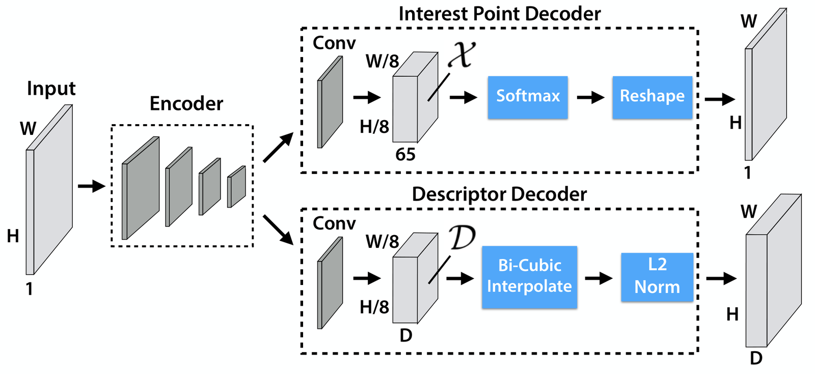
The encoder is a VGG-style stack that downsamples by 8. The detector head outputs, for every 8x8 cell, 65 logits: one per pixel position in the cell plus a "dustbin" for "no keypoint here". A softmax over those 65, with the dustbin dropped, gives a keypoint probability per pixel. The descriptor head outputs a dense 256-dimensional vector field at 1/8 resolution, bilinearly sampled and L2-normalized at each keypoint. Both heads read the same encoder features, so the representation and most of the compute are shared — the paper's whole point against detect-then- describe systems that "lack the ability to share computation". Train it self-supervised with Homographic Adaptation (warp an image by many homographies, detect in each, vote), and you get a detector that is repeatable across viewpoint and a descriptor you can match.

That is why it became the standard learned front-end. Its descriptors feed matchers like LightGlue and SuperGlue; its keypoints anchor visual SLAM and structure-from-motion. The interface is small and stable — grayscale in, keypoints and 256-d descriptors out — so it slots under a lot of geometry. The cost is that it is a convolutional network run per frame, and on an edge device that per-frame cost is the budget you fight.

PrunaSuperPoint is built on rpautrat/SuperPoint, Rémi Pautrat and Paul-Edouard Sarlin's implementation of that method, with weights converted from the original TensorFlow release. Its default config (measured, from superpoint.py) is channels = [64, 64, 128, 128, 256]: eight 3x3 convolutions in four blocks, a 2x pool after each of the first three blocks, then the two heads. Descriptor dimension 256, detector output 65.

Where the time actually goes

Here is the part that makes the pruning choices obvious instead of arbitrary. A convolution at spatial size $H' \times W'$ with $c_{\text{in}}$ input and $c_{\text{out}}$ output channels and a $k \times k$ kernel costs

multiply-accumulates. The spatial term is the trap. Block 0 runs at the full input resolution; block 1 at a quarter of the area, block 2 at a sixteenth, block 3 at a sixty-fourth. So an early layer with modest channel counts can dwarf a late layer with many channels, purely because it touches more pixels.

Run the arithmetic at 640x480 (measured, my count from the layer dimensions): backbone_0_1, the second convolution, is 64 channels in and out at full resolution — 11.3 GMACs, 49.6% of the entire eight-layer backbone on its own. The whole backbone is 22.8 GMACs; the two heads, running at 80x60, add 3.2 GMACs, for 26.1 GMACs a frame. The bottleneck is not where the channels are widest. It is where the pixels are.

That reframes "make SuperPoint faster" as "cut channels out of the first two convolutions, where each channel removed is paid at full resolution." The widget below is that arithmetic, live. Drag the bottleneck down, or pick a card variant, and watch the per-layer MACs and the totals move:

The ghost bars are the original layer costs; the filled bars are the current config. The heads sit at the bottom in grey because they are never touched — remember them, they are the reason the speedup is smaller than the compute saving.

Structural pruning, not masking

There are two kinds of pruning, and only one of them is faster on real hardware.

Unstructured pruning zeroes individual weights. You can zero 90% of a weight matrix and the layer still has the same shape; a dense convolution kernel still launches over the same tensor and does the same number of MACs. You save memory and, with sparse kernels and the right hardware, sometimes time — but a stock FP16 TensorRT conv on a Jetson runs the dense shape regardless of how many zeros you fed it.

Structural pruning removes whole channels. The layer gets physically smaller: fewer filters, a smaller output tensor, fewer MACs, and the next layer's input shrinks to match. That is what actually makes a dense conv faster, because the kernel now runs over a smaller tensor. The cost is that you cannot pick channels freely — removing a channel is removing a feature the next layer expected, so the network's accuracy drops until you repair it.

PrunaSuperPoint does the structural kind, and the code is unambiguous (measured, from models/superpoint.py, prune_backbone). To prune a layer's input to channel dimensions it scores each input channel by the mean absolute weight across all output filters and kernel positions — old2.weight.abs().mean(dim=(0, 2, 3)) — keeps the top-channel by that score, and then rebuilds two nn.Conv2d modules at the new size: the previous layer with fewer output filters, this layer with fewer input channels, copying the kept slices. The BatchNorm in between is resized to match. Nothing is masked; the modules are genuinely smaller afterward.

Keeping the highest-magnitude channels is a heuristic, not a proof — a small weight can still carry a useful feature — but the card states its real purpose plainly: it "provides a good initialization point for potential distillation training." The pruning picks a decent starting network; the training that follows is what makes it good.

The config Pruna ships, 16_16_24_32_64.ckpt, prunes the first six layers (measured): the chain of backbone output widths goes from [64, 64, 64, 64, 128, 128, …] to [16, 16, 24, 32, 64, 128, …]. By my arithmetic that is 4.8x fewer backbone MACs (22.8 to 4.7 GMACs) and 3.3x across the whole network (26.1 to 8.0 GMACs) — the figures the widget prints for the pruned variant. backbone_0_1 alone falls from 11.3 to 0.7 GMACs, a 16x cut in the single most expensive layer.

Why it needs distillation

Prune six layers down to a quarter of their width and the network is broken — it has the right shape and reasonable initial filters, but it has never been trained to produce good keypoints at that size. The card shows exactly how broken, and it is the most instructive pair of rows in the table.

pruned-light prunes only the bottleneck, backbone_0_1's input from 64 to 32 channels, with no training at all. On the indoor trace its keypoint coverage drops to 637 of 1024, and its mean descriptor L2 difference against the original is 0.92 (reported). That is one layer, lightly pruned, and the descriptors have already drifted badly.

pruned prunes six layers, far more aggressively, but then runs a short distillation. Its coverage is 817 of 1024 and its descriptor difference 0.24 (reported) — better on both axes than the barely-pruned, untrained model. More pruning, better quality, because of the training in between. That is the entire argument for distillation in one comparison: the pruned network is a student, and a few hundred frames of the original model's own outputs teach it to behave like the teacher at a fraction of the width.

The distillation is deliberately small (measured, from distillation/base_config.yaml and losses.py): 250 frames from the UZH-FPV indoor trace, 300 epochs, and a three-term loss. The detector is supervised two ways against the frozen original — a cross-entropy on the teacher's argmax keypoint cells and a KL divergence on the teacher's softened 65-way distribution (the config weights both at 2.0). The descriptor head gets a cosine-similarity loss, 1 - cos, pulling the student's descriptor at each location toward the teacher's (weight 1.0). KL and cosine are the right tools here: you are not training against ground-truth labels, you are copying a model you trust, so you match its distribution and its descriptor directions, not a hard target.

expand

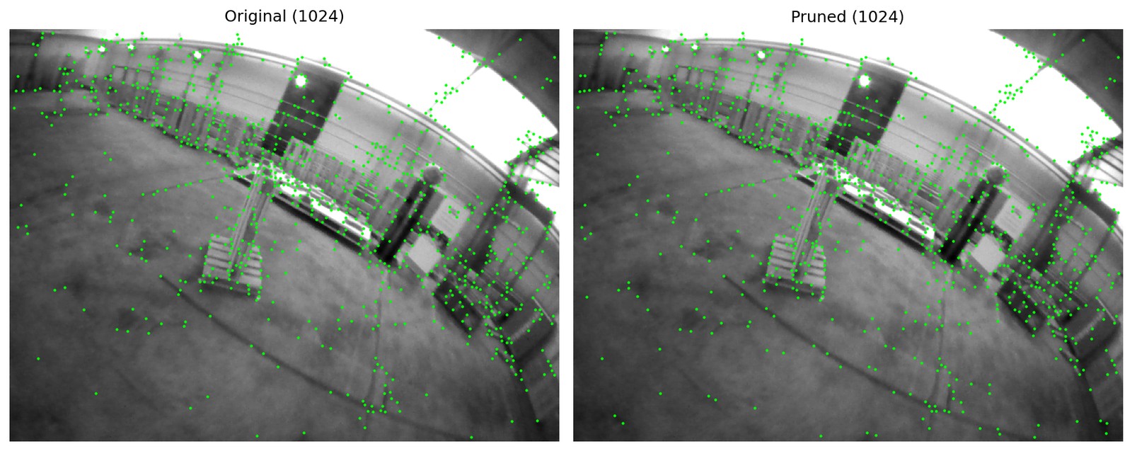
Coverage looks preserved at a glance, and it mostly is — but the metric is spatial distribution over 8x8 regions, not exact agreement. The next figure is the honest version: where the two models' keypoints actually coincide.

expand

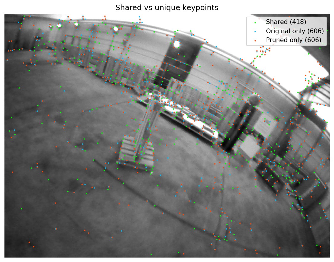
Only 418 of about 1024 keypoints are detected at the exact same pixel. The card is candid about this — "relatively few exact overlaps, many predictions lie very close" — and it matters for a downstream matcher, which cares about repeatability across frames more than agreement with the teacher. The card does not test a downstream task, and says so. That is the right caveat: a pruned front-end should be judged inside the SLAM or SfM pipeline it feeds, not only against the original's keypoint set.

Hierarchical top-k, and skipping the refinement

Two more optimizations are about keypoint selection, after the network has run.

To keep the top $k$ keypoints by score, the obvious thing is a global top-k over the whole heatmap. On a constrained device that is a poor fit — a single large selection does not parallelize well. PrunaSuperPoint does it hierarchically (measured, hierarchical_topk): split the score map into chunks, take the top $k$ from each chunk, then take the top $k$ of the pooled candidates. The card uses 32 chunks at 640x480 and 36 at 1080p (reported).

The thing I like about this one is that it is exact, not an approximation, and the reason is a clean little argument. The global top-$k$ are the $k$ highest scores anywhere. Restrict them to any one chunk: that chunk can contain at most $k$ of them, and the chunk's own top-$k$ already holds its $k$ highest scores, so it contains every global winner that falls inside it. The union of all chunks' top-$k$ therefore contains the global top-$k$, and a final top-$k$ over that union recovers it exactly — assuming the same $k$ and no score ties. The card's original-topk row confirms it empirically: identical coverage (1024) and zero descriptor difference to the original, with a small speedup (17.0 vs 17.8 ms at 640x480, reported). A faster path to the same answer, which is rarer than it sounds.

The last one is a genuine trade, not a free lunch. After non-maximum suppression, the base model runs two refinement iterations to recover high-scoring keypoints that NMS suppressed — and each iteration is two max-pools over the full-size heatmap, so refinement is four extra full-resolution passes (measured, batched_nms). The pruned-noref variant skips them: at 640x480 it drops from 9.6 to 8.3 ms (reported), but indoor coverage falls from 817 to 700. Cheaper, with fewer keypoints recovered. Whether that is worth it "depends on the task", as the card puts it — which is the correct answer.

The evidence, and the gap

The latency table is the reason to care, and it is clean (reported, Jetson Orin Nano 8GB, FP16 TensorRT, our-benchmark figures):

Now the gap, which is the engineer's lesson in this release. I counted a 3.3x reduction in whole-network MACs for the pruned config. The measured latency improvement is 2.07x at 1080p and 1.98x at 640x480. Compute fell three and a third times; the wall clock fell two. Where did the other third go?

It went into the floor. The two heads do not shrink — they run at 80x60 on the unpruned 128-channel backbone output, 3.2 GMACs that stay fixed no matter how hard you prune the backbone. NMS and the top-k run on the full-size heatmap and do not scale with backbone width either. Memory traffic, kernel-launch overhead and the fixed-cost stages set a latency floor, and once the backbone is cheap enough, you are paying mostly for that floor. You can see it in the other direction too: pruned-light removes only full-resolution compute and its latency falls almost in step with its MACs (1.28x MACs, ~1.24x latency, reasoned against reported), because the work it removes is exactly the expensive kind. Prune deeper and you win more compute but less of it converts to time. This is the usual shape of inference optimization, and it is why FLOPs are a lead indicator, never a promise.

The quality side, read honestly: the distilled pruned model keeps 817/1024 coverage indoors and 754 outdoors, with descriptor L2 differences of 0.24 and 0.27 (reported) — strong, given a third of the compute and a 250-frame recovery run that never saw the outdoor trace. It is not free: the descriptors are close to but not identical to the original's, so a matcher tuned on original SuperPoint descriptors will see shifted inputs, and the card's own first limitation is that it has not been evaluated in a downstream task.

What is preserved, and what it costs

The architecture PrunaSuperPoint exposes is unchanged: grayscale in, a 65-logit detector map and a 256-d descriptor map out, stride 8, same two-head design. Only the inside changes — a narrower backbone and distilled weights — so the exported ONNX and TensorRT engine drop into a pipeline where the original sat, which is the property that makes it useful. "Drop-in" is true at the interface, with the caveat above that the descriptors are near, not equal.

Where it costs, stated plainly:

• Interface, not weights. You cannot load the pruned checkpoint into the original graph; it is a differently-shaped, separately-trained network. Drop-in means same inputs and outputs, not same weights.
• No downstream number. The card reports keypoint coverage and descriptor difference, not pose error or map quality in a SLAM run. The right test, which it names as future work, is the task itself.
• Recovery data is thin and sequential. 250 frames from one indoor trace, and the outdoor numbers come from a model that never trained on outdoor data. It generalized, but 754 vs 817 coverage is the visible cost of the domain gap.
• Licensing of the matcher. The card notes it deliberately avoids the SuperPoint builds paired with LightGlue because of their restrictive licences; this release is Apache-2.0 and shows the method. To prune a LightGlue-paired SuperPoint you redo the structural surgery and a distillation run against your own config.

This sits next to the other compression work the site has covered from different angles: NVIDIA's Model Optimizer does structural pruning too, with Minitron's activation-magnitude importance over width and depth, plus distillation to recover; the LLM Compressor 0.14 piece covers the quantization side; and Pruna's own earlier work, the few-step Qwen-Image adapters, is the distillation-for-speed idea applied to diffusion rather than convnets. The target here is different — a per-frame perception front-end on a low-power edge board, not a server-side generative model — and the win is engineered to the hardware: cut the full-resolution convolutions, recover with a teacher, and leave the interface alone so the rest of the stack, the matcher and the SLAM backend in something like SurfSLAM or a LiDAR-inertial system like FAR-LIO, never has to know.

The one-paragraph version

PrunaSuperPoint makes SuperPoint faster by pruning where SuperPoint spends its time: the first convolutions, which run at full resolution and hold half the backbone's compute. It removes whole channels (structural, so a dense FP16 conv genuinely runs smaller), keeping the highest-magnitude ones as a starting point, then distills the narrow student against the original with a KL + cross-entropy detector loss and a cosine descriptor loss over 250 frames — which is what turns a broken pruned network (637 coverage, 0.92 descriptor drift) into a usable one (817, 0.24). A hierarchical top-k returns the exact same keypoints faster, and skipping NMS refinement trades four full-resolution passes for a few fewer keypoints. The result is a reported ~2.1x on a Jetson Orin Nano at 1080p from a reasoned 3.3x compute cut — the difference being the unpruned heads and the selection stages, the fixed floor that no amount of backbone pruning touches. The architecture is preserved at the interface, so it drops in; the descriptors are close but not identical, and the right place to judge it is the downstream task the card honestly declines to run.